Using a DESC Equilibrium Output

This tutorial covers computing quantities of interest in DESC, plotting, and interfacing with external codes that expect a VMEC-like output file.

import sys
import os
import matplotlib.pyplot as plt

plt.rcParams.update({"font.size": 18})
sys.path.insert(0, os.path.abspath("."))
sys.path.append(os.path.abspath("../../../"))

Loading in a DESC Equilibrium

DESC saves its output files as .h5 files, which can be loaded using the load function contained in the desc.io module

import desc.io

DESC version 0.10.2+284.gc431037d.dirty,using JAX backend, jax version=0.4.13, jaxlib version=0.4.13, dtype=float64
Using device: CPU, with 15.23 GB available memory

In DESC, equilibrium solutions are stored as Equilibrium objects, which contain the spectral coefficients of the solved equilibrium as well as the last-closed-flux-surface used to solve the equilibrium, the pressure and iota profiles, and other quantities that define the equilibrium.

Often in DESC, a continuation method is employed to solve for equilibria where a sequence of related equilibria are computed until the final resolution and input parameters are reached. When calling DESC from the command line, this sequence of Equilibrium objects are stored inside an EquilibriaFamily object, which essentially acts as a list of Equilibrium objects with some extra functionality to aid in the continuation method.

We will load in the solution to the HELIOTRON example input file we solved in the previous notebook now.

eq_fam = desc.io.load("input.HELIOTRON_output.h5")
print(type(eq_fam))

<class 'desc.equilibrium.equilibrium.EquilibriaFamily'>

As you can see, the object we just loaded in is an EquilibriaFamily. We can check to see how many equilibria this family contains (3, each corresponding to a different step in the continuation method outlined in the HELIOTRON input file).

len(eq_fam)

8

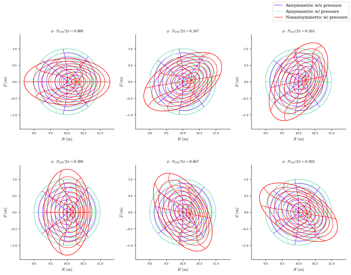
We can visualize the different equilibria with the plot_comparison function, which plots flux surfaces and the contours of constant straight field-line poloidal angle \(\vartheta=\theta+\lambda\) for multiple equilibria.

%matplotlib inline
from desc.plotting import plot_comparison

fig, ax = plot_comparison(
    eqs=[eq_fam[1], eq_fam[3], eq_fam[-1]],
    labels=[
        "Axisymmetric w/o pressure",
        "Axisymmetric w/ pressure",
        "Nonaxisymmetric w/ pressure",
    ],
)

Computing Quantities from a DESC Equilibrium

Now let’s focus on a single equilibrium. We can choose the final solution by indexing the last element of eq_fam

eq = eq_fam[-1]
print(type(eq))

<class 'desc.equilibrium.equilibrium.Equilibrium'>

Notice now we have an Equilibrium object, not an EquilibriaFamily. Printing an Equilibrium will list some information about it

print(eq)

Equilibrium at 0x7f3d79000970 (L=8, M=8, N=3, NFP=19, sym=1, spectral_indexing=ansi)

Here we can see that this equilibrium solution has 19 field periods (NFP=19) and is represented with a Fourier-Zernike spectral basis with radial resolution of L=8, poloidal resolution of M=8, and toroidal resolution of N=3. It is stellarator symmetric (sym=1), and the spectral indexing scheme used for the Zernike Polynomial basis was the ansi indexing (for more information on the indexing schemes see the DESC documentation).

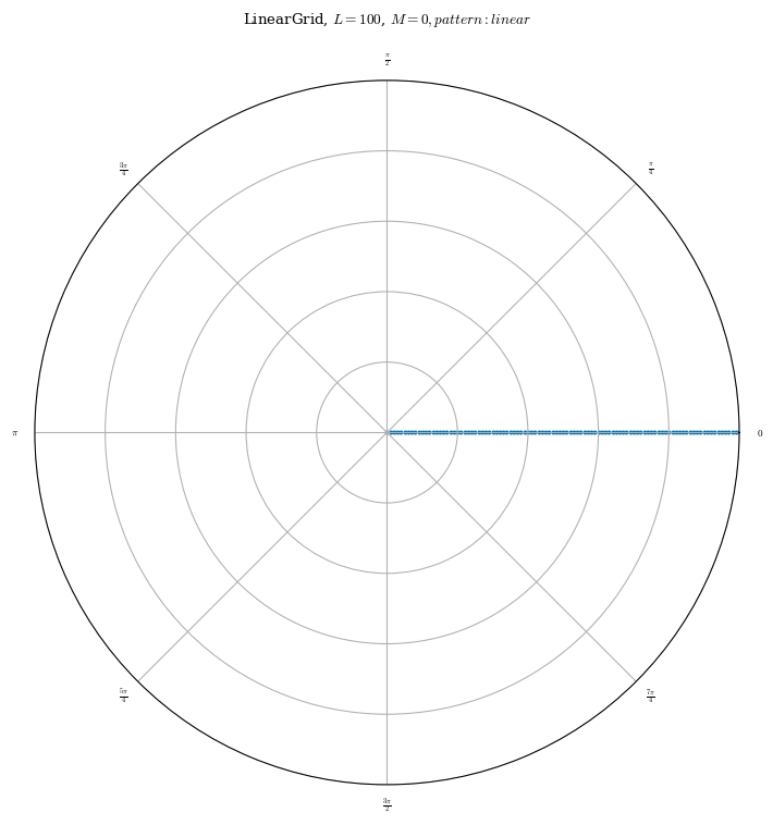
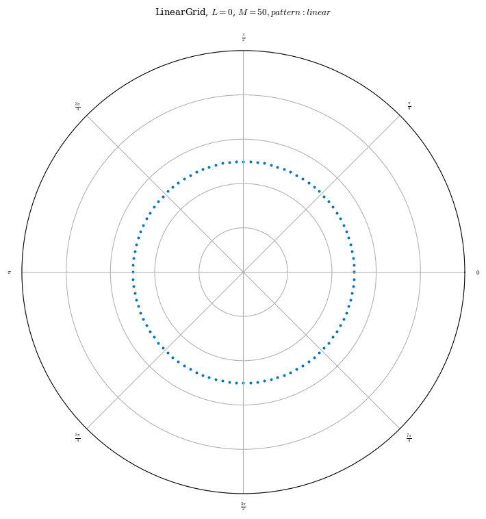
Grids in DESC are objects from the desc.grid module which specify points in computational space \((\rho,\theta,\zeta)\). We typically want to plot at linearly spaced points, so we will use the LinearGrid class to make a 1-dimensional grid of points linearly spaced in \(\rho\).

grid.nodes shows the points in the grid, each element being \((\rho,\theta,\zeta)\). Notice our grid is an array of points from \(\rho=0\) to \(\rho=1\) equally spaced, all at \(\theta=\zeta=0\).

from desc.grid import LinearGrid

grid_1d = LinearGrid(L=100)  # 101 linearly-spaced radial grid points
grid_1d.nodes[:10, :]  # show the first 10

array([[0.  , 0.  , 0.  ],
       [0.01, 0.  , 0.  ],
       [0.02, 0.  , 0.  ],
       [0.03, 0.  , 0.  ],
       [0.04, 0.  , 0.  ],
       [0.05, 0.  , 0.  ],
       [0.06, 0.  , 0.  ],
       [0.07, 0.  , 0.  ],
       [0.08, 0.  , 0.  ],
       [0.09, 0.  , 0.  ]])

We can visualize the grid using the plot_grid function.

from desc.plotting import plot_grid

plot_grid(grid_1d, figsize=(8, 8));

Equilibrium objects have a compute method which can be used to compute many useful quantities (a full list of which can be found in the DESC docs) that are commonly needed from an equilibrium.

The compute method takes as arguments the name (as a string) of the desired quantity and the grid you wish the quantity to be computed on. It then returns a dictionary containing that quantity, as well as all the intermediate quantities needed to compute the desired quantity.

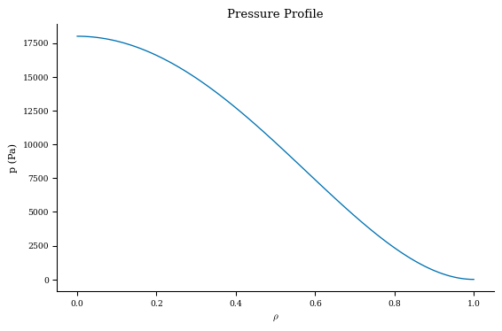
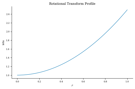
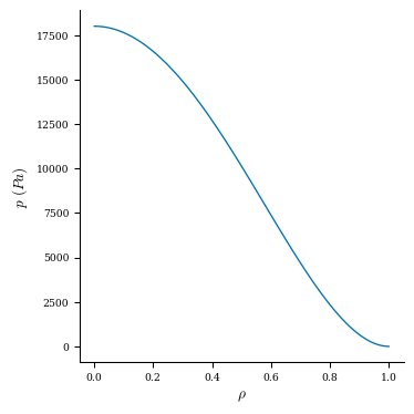
As an example, let’s plot the pressure and rotational transform profiles of this equilibrium.

pressure_data = eq.compute("p", grid=grid_1d)
iota_data = eq.compute("iota", grid=grid_1d)

pressure_data.keys()

dict_keys(['Ti', 'Te', 'Zeff', 'ne', 'p'])

iota_data.keys()

dict_keys(['iota_den', 'rho', 'psi_r', 'psi_rr', 'iota_den_r', 'iota_num vacuum', 'iota_num current', 'iota_num', 'iota_num_r vacuum', 'iota_num_r current', 'iota_num_r', 'iota'])

Notice that the returned dictionary for iota has more than just iota as a key. Generally, eq.compute will return the desired quantity along with each of its dependencies needed to calculate that quantity. Don’t rely on this, to ensure that you get all the quantities you need, it is better to pass in explicitly each quantity, for example you want both p and p_r, you must call eq.compute(["p","p_r"]).

(NOTE: pressure_data also contains kinetic profiles, but these are NaN unless the equilibrium was specifically given kinetic profiles, so we will ignore that output for now)

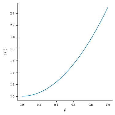
Let’s plot the profiles now:

import matplotlib.pyplot as plt

p = pressure_data["p"]
iota = iota_data["iota"]

plt.figure()
plt.plot(grid_1d.nodes[:, 0], p)
plt.title("Pressure Profile")
plt.xlabel(r"$\rho$")
plt.ylabel("p (Pa)")

plt.figure()
plt.plot(grid_1d.nodes[:, 0], iota)
plt.title("Rotational Transform Profile")
plt.xlabel(r"$\rho$")
plt.ylabel("iota")

Text(0, 0.5, 'iota')

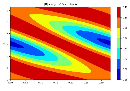
Now let’s compute the magnetic field strength on the \(\rho=0.5\) surface.

When making the grid we will specify that we want poloidal and toroidal grid points using \(M\) and \(N\), but only at the \(\rho=0.5\) surface. Adding the NFP argument to the grid will ensure we have toroidal points only for a single field period.

import numpy as np

# integer inputs specify the number of grid points in that dimension
# according to the formula npts =  2*integer + 1
# float or ndarray of floats specify the coordinate values directly
grid_2d_05 = LinearGrid(rho=np.array(0.5), M=50, N=50, NFP=eq.NFP, endpoint=True)
plot_grid(grid_2d_05, figsize=(8, 8));

Notice now that we have grid points at \(\rho=0.5\) and \(0\leq\theta<2\pi\) and \(0\leq\zeta<\frac{2\pi}{NFP}\)

mod_B_data = eq.compute("|B|", grid=grid_2d_05)

We can look at the returned dictionary now and see that all the intermediate quantities necessary to calculate |B| are also returned (the magnetic field contravariant components, basis vectors, iota, etc.)

mod_B_data.keys()

dict_keys(['iota_den', 'iota_num vacuum', 'rho', 'psi_r', 'iota_num current', 'iota_num', 'iota', 'R', 'R_r', 'Z_r', '0', 'omega_r', 'e_rho', 'R_t', 'Z_t', 'omega_t', 'e_theta', 'R_z', 'Z_z', 'omega_z', 'e_zeta', 'sqrt(g)', 'B0', 'lambda_z', 'B^theta', 'lambda_t', 'B^zeta', 'B', '|B|^2', '|B|'])

mod_B = mod_B_data["|B|"]

To plot this 2d data, it is important to understand that in DESC all quantities and grid points are by default in a single stack. If we look at the shape of grid_2d_05.nodes, we can see that it is 10,201 nodes (1 \(\rho\) coordinate x 101 \(\theta\) coordinates x 101 \(\zeta\) coordinates), each of length 3 \((\rho,\theta,\zeta)\). Similarly, mod_B is given at these 10,201 nodes.

grid_2d_05.nodes.shape

(10201, 3)

mod_B.shape

(10201,)

To plot this, we must reshape it into a 2D array as follows

# reshape to form grids for plotting
zeta = (
    grid_2d_05.nodes[:, 2]
    .reshape((grid_2d_05.num_theta, grid_2d_05.num_rho, grid_2d_05.num_zeta), order="F")
    .squeeze()
)
theta = (
    grid_2d_05.nodes[:, 1]
    .reshape((grid_2d_05.num_theta, grid_2d_05.num_rho, grid_2d_05.num_zeta), order="F")
    .squeeze()
)
mod_B = mod_B.reshape(
    (grid_2d_05.num_theta, grid_2d_05.num_rho, grid_2d_05.num_zeta), order="F"
)

# plot contours of |B| on the rho=0.5 surface
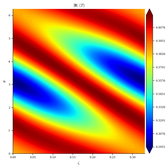
plt.contourf(zeta, theta, mod_B[:, 0, :], cmap="jet")
plt.xlabel(r"$\zeta$")
plt.ylabel(r"$\theta$")
plt.title(r"$|\mathbf{B}|$ on $\rho=0.5$ surface")
plt.colorbar()

<matplotlib.colorbar.Colorbar at 0x7f3b1055e110>

Hopefully the process of computing quantities from a DESC equilibrium is clearer now. A full list of the quantities available for computation already in DESC is given in the DESC documentation

Plotting Utilities In DESC

For normal plotting needs, DESC has an extensive array of plotting utilities that can be used to quickly plot quantities of interest.

from desc.plotting import plot_1d, plot_2d, plot_3d, plot_section, plot_boozer_surface

fig, ax = plot_1d(eq, "p")  # default grid is linearly spaced in rho
fig, ax = plot_1d(eq, "iota")
fig, ax = plot_2d(eq, "|B|", grid=grid_2d_05)  # plot |B| on rho=0.5 surface

fig = plot_3d(eq, "|B|")
fig.show()
# note that this example has 19 toroidal field periods

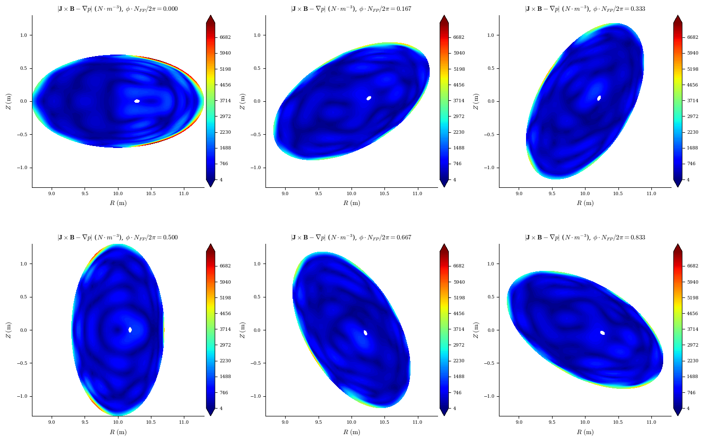
fig, ax = plot_section(eq, "|F|")  # plot force error

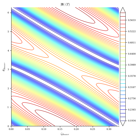
# |B| in Boozer coordinates on the rho=0.7 surface
fig, ax = plot_boozer_surface(
    eq, grid_plot=LinearGrid(rho=np.array(0.7), M=50, N=50, NFP=eq.NFP, endpoint=True)
)

Each of the plotting routines takes additional arguments that can be used to customize the appearance of the plots, full details can be found in the documentation.

Also note that each plotting function (with the sole exception of plot_3d, which uses plotly) returns a handle to the Matplotlib figure and a numpy array of the axes used. These can then be further modified to customize the appearance of the plots.

Saving To VMEC-Formatted Output

# used to save equilibrium objects as VMEC-formatted .nc files
from desc.vmec import VMECIO

from desc.plotting import plot_surfaces, plot_section

In this example, we will use a precomputed equilibria from desc.examples

import desc.examples

eq = desc.examples.get("SOLOVEV")

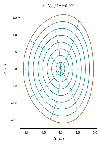
We can look at the final flux surfaces using the plot_surfaces function, and the final normalized force error with the plot_section function, both from desc.plotting:

plot_surfaces(eq);

No artists with labels found to put in legend.  Note that artists whose label start with an underscore are ignored when legend() is called with no argument.

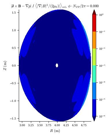
# we want to plot the magnitude of the force error |F|, and we want it shown normalized by the pressure gradient
plot_section(eq, name="|F|", norm_F=True, log=True);

To save the equilibrium in a VMEC-formatted .nc file, we use the VMECIO class we imported from desc.vmec. This class will convert the quantities defining the equilibrium from DESC coordinates to VMEC equivalents.

VMECIO.save(eq, "./SOLOVEV_output.nc")

Saving parameters
Saving R
Saving Z
Saving lambda
Saving Jacobian
Saving |B|
Saving B^theta
Saving B^zeta
Saving B_psi
Saving B_theta
Saving B_zeta
Saving J^theta*sqrt(g)

/home/fouriest/SCHOOL/Princeton/PPPL/DESC/desc/vmec_utils.py:89: RuntimeWarning:

invalid value encountered in matmul

Saving J^zeta*sqrt(g)

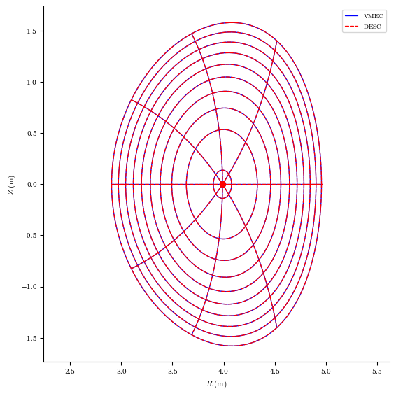
We now have a file SOLOVEV_output.nc which is the equivalent Equilibrium solution in the VMEC coordinates and data format. We can now treat it as any other VMEC .nc file. For example, we can use our VMEC comparison tools to compare the two files now, such as comparing the flux surfaces using VMECIO.plot_vmec_comparison (which unsurprisingly are the same):

vmec_formatted_eq_file = "./SOLOVEV_output.nc"
VMECIO.plot_vmec_comparison(eq, vmec_formatted_eq_file);