Near axis constraints
This tutorial shows how to find equilibrium solutions in DESC which are constrained to have the same axis and near-axis behavior as a NAE solution from the pyQSC or pyQIC codes
Creating a DESC Equilibrium from a pyQSC or pyQIC Near-Axis Equilibrium
Note that you must have pyQSC and/or pyQIC installed in order to make use of the Equilibrium.from_near_axis method. You can do so with pip install qsc.
If you have access to a GPU, uncomment the following two lines before any DESC or JAX related imports. You should see about an order of magnitude speed improvement with only these two lines of code!
[ ]:
# from desc import set_device
# set_device("gpu")
As mentioned in DESC Documentation on performance tips, one can use compilation cache directory to reduce the compilation overhead time. Note: One needs to create jax-caches folder manually.
[3]:
# import jax

# jax.config.update("jax_compilation_cache_dir", "../jax-caches")
# jax.config.update("jax_persistent_cache_min_entry_size_bytes", -1)
# jax.config.update("jax_persistent_cache_min_compile_time_secs", 0)
[4]:
# must have installed pyQsc with `pip install qsc` in order to use this!
from qsc import Qsc
import numpy as np
import matplotlib.pyplot as plt
from desc.equilibrium import Equilibrium
from desc.objectives import get_fixed_boundary_constraints
from desc.plotting import (
    plot_comparison,
    plot_fsa,
    plot_section,
    plot_surfaces,
    plot_qs_error,
)
DESC is able to create an equilibrium based off of a pyQsc NAE equilibrium object. First, we’ll make the NAE equilibrium using pyQsc
[5]:
qsc_eq = Qsc.from_paper("precise QA")
Then, to make the DESC equilibrium, the Equilibrium class has a method Equilibrium.from_near_axis. This method creates a DESC Equilibrium based off of the pyQsc equilibrium. It requires as input the desired DESC Fourier-Zernike resolutions, as well as the radius at which you want to evaluate the qsc equilibrium at to make the DESC equilibrium’s boundary. The equilibrium’s initial R_lmn, Z_lmn Fourier-Zernike coefficients are fit to the R,Z evaluated from the Qsc
equilibrium, and the initial L_lmn are 0 (because the Qsc equilibrium uses Boozer angles, so there is no poloidal stream function)
[6]:
# ntheta is the number of points in theta to sample
# when fitting the DESC Fourier-Zernike basis to
# the NAE surfaces.
# The more shaped the NAE surfaces, the higher this should be,
# 75 is a good minimum value.
ntheta = 75
# r is the finite radius to evaluate the NAE surfaces at, this will
# roughly set the aspect ratio of the resulting solution.
# However if this is too large, the surfaces from the NAE may become
# self-intersecting! The r at which this occurs varies for different NAE
# solutions, r=0.35 was found to be a reasonable radius for precise QA
r = 0.35
eq_fixed_bdry = Equilibrium.from_near_axis(
    qsc_eq,  # the Qsc equilibrium object
    r=r,  # the finite radius (m) at which to evaluate the Qsc surface to use as the DESC boundary
    L=8,  # DESC radial resolution
    M=8,  # DESC poloidal resolution
    N=8,  # DESC toroidal resolution
    ntheta=ntheta,
)
eq_fit = eq_fixed_bdry.copy()  # copy so we can see the original Qsc surfaces later
Now we solve the equilibrium as normal in DESC
[7]:
# get the fixed-boundary constraints, which include also fixing the pressure and fixing the current profile (iota=False flag means fix current)
constraints = get_fixed_boundary_constraints(eq=eq_fixed_bdry)
for c in constraints:
    print(c.__class__.__name__)

# solve the equilibrium
eq_fixed_bdry.solve(
    verbose=3,
    ftol=1e-2,
    objective="force",
    maxiter=100,
    xtol=1e-6,
    constraints=constraints,
)

# Save equilibrium as .h5 file
eq_fixed_bdry.save("DESC_from_NAE_precise_QA_output.h5")
FixBoundaryR
FixBoundaryZ
FixPsi
FixPressure
FixCurrent
FixSheetCurrent
Building objective: force
Precomputing transforms
Timer: Precomputing transforms = 745 ms
Timer: Objective build = 1.12 sec
Building objective: lcfs R
Building objective: lcfs Z
Building objective: fixed Psi
Building objective: fixed pressure
Building objective: fixed current
Building objective: fixed sheet current
Building objective: self_consistency R
Building objective: self_consistency Z
Building objective: lambda gauge
Building objective: axis R self consistency
Building objective: axis Z self consistency
Timer: Objective build = 338 ms
Timer: LinearConstraintProjection build = 4.87 sec
Number of parameters: 856
Number of objectives: 5346
Timer: Initializing the optimization = 6.47 sec

Starting optimization
Using method: lsq-exact
Solver options:
------------------------------------------------------------
Maximum Function Evaluations       : 501
Maximum Allowed Total Δx Norm      : inf
Scaled Termination                 : True
Trust Region Method                : qr
Initial Trust Radius               : 1.207e+02
Maximum Trust Radius               : inf
Minimum Trust Radius               : 2.220e-16
Trust Radius Increase Ratio        : 2.000e+00
Trust Radius Decrease Ratio        : 2.500e-01
Trust Radius Increase Threshold    : 7.500e-01
Trust Radius Decrease Threshold    : 2.500e-01
------------------------------------------------------------

   Iteration     Total nfev        Cost      Cost reduction    Step norm     Optimality
       0              1          1.177e+01                                    4.040e+00
       1              2          3.209e+00      8.557e+00      4.955e-01      1.777e+00
       2              3          1.034e-01      3.105e+00      1.833e-01      1.785e-01
       3              4          1.443e-02      8.898e-02      1.385e-01      5.654e-02
       4              5          1.296e-02      1.473e-03      2.225e-01      7.653e-02
       5              6          1.062e-03      1.190e-02      5.777e-02      7.885e-03
       6              8          7.625e-04      2.991e-04      4.662e-02      5.554e-03
       7              9          7.341e-04      2.837e-05      6.297e-02      8.131e-03
       8             10          6.160e-04      1.181e-04      2.099e-02      3.481e-04
       9             11          6.002e-04      1.586e-05      3.258e-02      1.048e-03
      10             12          5.806e-04      1.959e-05      2.117e-02      7.978e-04
      11             14          5.699e-04      1.068e-05      9.295e-03      1.766e-04
      12             15          5.621e-04      7.784e-06      1.646e-02      6.362e-04
      13             17          5.561e-04      6.039e-06      8.049e-03      1.360e-04
      14             18          5.506e-04      5.524e-06      1.656e-02      4.609e-04
Optimization terminated successfully.
`ftol` condition satisfied. (ftol=1.00e-02)
         Current function value: 5.506e-04
         Total delta_x: 3.306e-01
         Iterations: 14
         Function evaluations: 18
         Jacobian evaluations: 15
Timer: Solution time = 13.8 sec
Timer: Avg time per step = 922 ms
==============================================================================================================
                                                                 Start  -->   End
Total (sum of squares):                                      1.177e+01  -->   5.506e-04,
Maximum absolute Force error:                                9.225e+06  -->   3.812e+04 (N)
Minimum absolute Force error:                                1.773e+00  -->   9.709e-02 (N)
Average absolute Force error:                                7.598e+04  -->   8.515e+02 (N)
Maximum absolute Force error:                                4.467e+00  -->   1.846e-02 (normalized)
Minimum absolute Force error:                                8.585e-07  -->   4.701e-08 (normalized)
Average absolute Force error:                                3.679e-02  -->   4.123e-04 (normalized)
R boundary error:                                            0.000e+00  -->   7.889e-17 (m)
Z boundary error:                                            0.000e+00  -->   5.710e-17 (m)
Fixed Psi error:                                             0.000e+00  -->   0.000e+00 (Wb)
Fixed pressure profile error:                                0.000e+00  -->   0.000e+00 (Pa)
Fixed current profile error:                                 0.000e+00  -->   0.000e+00 (A)
Fixed sheet current error:                                   0.000e+00  -->   0.000e+00 (~)
==============================================================================================================
Now we have a DESC equilibrium solved with the boundary from Qsc. It has zero toroidal current as its profile constraint along with zero pressure since the original Qsc equilibrium had no pressure or current.
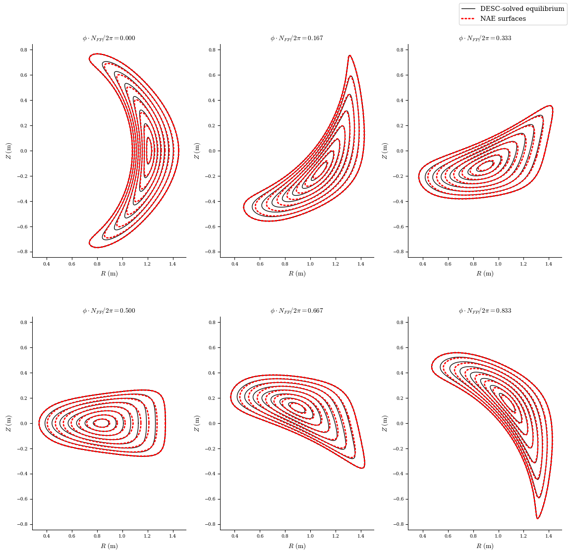
However, if we plot the surfaces, we see that while the boundary matches, the interior deviates slightly from the NAE, especially near the core. This means we may have lost some of the optimized properties from the QSC equilibrium.
[8]:
plot_comparison(
    eqs=[eq_fixed_bdry, eq_fit],
    labels=["DESC-solved equilibrium", "NAE surfaces"],
    figsize=(12, 12),
    theta=0,
    color=["k", "r"],
    ls=["-", ":"],
    lw=[1, 2],
);
Instead of evaluating the NAE at a finite radius, fixing that boundary, and hoping the axis behavior stays the same, we can instead directly fix the axis and the \(O(\rho)\) asymptotic behavior.
Solving Equilibria with Fixed Axis and Fixed NAE \(O(\rho)\) Behavior in DESC
[9]:
# utility functions for getting the NAE constraints
from desc.objectives import (
    get_equilibrium_objective,
    get_NAE_constraints,
    FixNearAxisR,
    FixNearAxisZ,
    FixPressure,
    FixCurrent,
    FixPsi,
)

eq_NAE = eq_fit.copy()
# the constraints we want are:
constraints = (
    FixNearAxisR(eq_NAE, target=qsc_eq, order=1),
    FixNearAxisZ(eq_NAE, target=qsc_eq, order=1),
    FixPressure(eq_NAE),
    FixCurrent(eq_NAE),
    FixPsi(eq_NAE),
)

# Alternatively, we can use the util function:
constraints = get_NAE_constraints(eq_NAE, qsc_eq, order=1)
for c in constraints:
    print(c.__class__.__name__)


eq_NAE.solve(
    verbose=3,
    ftol=1e-2,
    objective="force",
    maxiter=25,
    xtol=1e-6,
    constraints=constraints,
);
FixPsi
FixPressure
FixCurrent
FixSheetCurrent
FixNearAxisR
FixNearAxisZ
Building objective: force
Precomputing transforms
Timer: Precomputing transforms = 68.0 ms
Timer: Objective build = 88.8 ms
Building objective: fixed Psi
Building objective: fixed pressure
Building objective: fixed current
Building objective: fixed sheet current
Building objective: Fix Near Axis R Behavior
Building objective: Fix Near Axis Z Behavior
Building objective: self_consistency R
Building objective: self_consistency Z
Building objective: lambda gauge
Building objective: axis R self consistency
Building objective: axis Z self consistency
Timer: Objective build = 1.43 sec
Timer: LinearConstraintProjection build = 2.30 sec
Number of parameters: 1094
Number of objectives: 5346
Timer: Initializing the optimization = 3.91 sec

Starting optimization
Using method: lsq-exact
Solver options:
------------------------------------------------------------
Maximum Function Evaluations       : 126
Maximum Allowed Total Δx Norm      : inf
Scaled Termination                 : True
Trust Region Method                : qr
Initial Trust Radius               : 1.588e+02
Maximum Trust Radius               : inf
Minimum Trust Radius               : 2.220e-16
Trust Radius Increase Ratio        : 2.000e+00
Trust Radius Decrease Ratio        : 2.500e-01
Trust Radius Increase Threshold    : 7.500e-01
Trust Radius Decrease Threshold    : 2.500e-01
------------------------------------------------------------

   Iteration     Total nfev        Cost      Cost reduction    Step norm     Optimality
       0              1          1.177e+01                                    4.040e+00
       1              4          1.978e+00      9.789e+00      2.645e-01      1.181e+00
       2              5          1.928e-01      1.785e+00      1.222e-01      2.735e-01
       3              6          3.588e-02      1.569e-01      1.264e-01      9.484e-02
       4              7          1.663e-02      1.925e-02      1.217e-01      4.963e-02
       5              8          1.166e-03      1.547e-02      7.140e-02      9.755e-03
       6             10          1.703e-04      9.954e-04      2.844e-02      3.224e-03
       7             12          2.774e-05      1.425e-04      1.632e-02      2.133e-03
       8             14          7.419e-07      2.700e-05      7.490e-03      2.093e-04
       9             16          3.329e-07      4.089e-07      3.166e-03      8.458e-05
      10             18          2.677e-07      6.526e-08      1.533e-03      1.610e-05
      11             19          2.504e-07      1.725e-08      2.976e-03      4.187e-05
      12             20          2.173e-07      3.312e-08      2.976e-03      3.245e-05
      13             21          1.915e-07      2.585e-08      2.969e-03      3.146e-05
      14             22          1.667e-07      2.471e-08      2.989e-03      2.800e-05
      15             23          1.443e-07      2.243e-08      3.021e-03      2.628e-05
      16             24          1.266e-07      1.774e-08      3.043e-03      3.049e-05
      17             25          1.139e-07      1.270e-08      3.035e-03      3.325e-05
      18             26          1.045e-07      9.404e-09      2.985e-03      3.400e-05
      19             27          9.635e-08      8.130e-09      2.905e-03      3.355e-05
      20             28          8.909e-08      7.256e-09      2.833e-03      3.297e-05
      21             29          8.283e-08      6.259e-09      2.796e-03      3.311e-05
      22             30          7.770e-08      5.134e-09      2.794e-03      3.465e-05
      23             31          5.796e-08      1.974e-08      7.972e-04      2.432e-06
      24             32          5.680e-08      1.159e-09      1.457e-03      9.583e-06
      25             33          5.417e-08      2.635e-09      1.425e-03      9.897e-06
Warning: Maximum number of iterations has been exceeded.
         Current function value: 5.417e-08
         Total delta_x: 3.882e-01
         Iterations: 25
         Function evaluations: 33
         Jacobian evaluations: 26
Timer: Solution time = 21.2 sec
Timer: Avg time per step = 816 ms
==============================================================================================================
                                                                 Start  -->   End
Total (sum of squares):                                      1.177e+01  -->   5.417e-08,
Maximum absolute Force error:                                9.225e+06  -->   3.060e+02 (N)
Minimum absolute Force error:                                1.773e+00  -->   3.075e-03 (N)
Average absolute Force error:                                7.598e+04  -->   9.481e+00 (N)
Maximum absolute Force error:                                4.467e+00  -->   1.482e-04 (normalized)
Minimum absolute Force error:                                8.585e-07  -->   1.489e-09 (normalized)
Average absolute Force error:                                3.679e-02  -->   4.591e-06 (normalized)
Fixed Psi error:                                             0.000e+00  -->   0.000e+00 (Wb)
Fixed pressure profile error:                                0.000e+00  -->   0.000e+00 (Pa)
Fixed current profile error:                                 0.000e+00  -->   0.000e+00 (A)
Fixed sheet current error:                                   0.000e+00  -->   0.000e+00 (~)
Fixed-Near-Axis R Behavior error:                            4.929e-07  -->   2.672e-15 (m)
Fixed-Near-Axis Z Behavior error:                            6.400e-07  -->   2.614e-15 (m)
==============================================================================================================
[10]:
# to ensure equilibrium, we may also do a fixed-boundary solve to confirm the equilibrium is indeed an equilibrium
eq_NAE.solve(ftol=1e-4);
Building objective: force
Precomputing transforms
Building objective: lcfs R
Building objective: lcfs Z
Building objective: fixed Psi
Building objective: fixed pressure
Building objective: fixed current
Building objective: fixed sheet current
Building objective: self_consistency R
Building objective: self_consistency Z
Building objective: lambda gauge
Building objective: axis R self consistency
Building objective: axis Z self consistency
Number of parameters: 856
Number of objectives: 5346

Starting optimization
Using method: lsq-exact
Optimization terminated successfully.
`ftol` condition satisfied. (ftol=1.00e-04)
         Current function value: 3.483e-08
         Total delta_x: 9.109e-03
         Iterations: 12
         Function evaluations: 17
         Jacobian evaluations: 13
==============================================================================================================
                                                                 Start  -->   End
Total (sum of squares):                                      3.915e-08  -->   3.483e-08,
Maximum absolute Force error:                                3.060e+02  -->   2.779e+02 (N)
Minimum absolute Force error:                                3.075e-03  -->   1.178e-03 (N)
Average absolute Force error:                                9.481e+00  -->   8.923e+00 (N)
Maximum absolute Force error:                                1.260e-04  -->   1.144e-04 (normalized)
Minimum absolute Force error:                                1.266e-09  -->   4.848e-10 (normalized)
Average absolute Force error:                                3.903e-06  -->   3.673e-06 (normalized)
R boundary error:                                            0.000e+00  -->   5.157e-18 (m)
Z boundary error:                                            0.000e+00  -->   3.204e-17 (m)
Fixed Psi error:                                             0.000e+00  -->   0.000e+00 (Wb)
Fixed pressure profile error:                                0.000e+00  -->   0.000e+00 (Pa)
Fixed current profile error:                                 0.000e+00  -->   0.000e+00 (A)
Fixed sheet current error:                                   0.000e+00  -->   0.000e+00 (~)
==============================================================================================================
Comparing near axis behavior
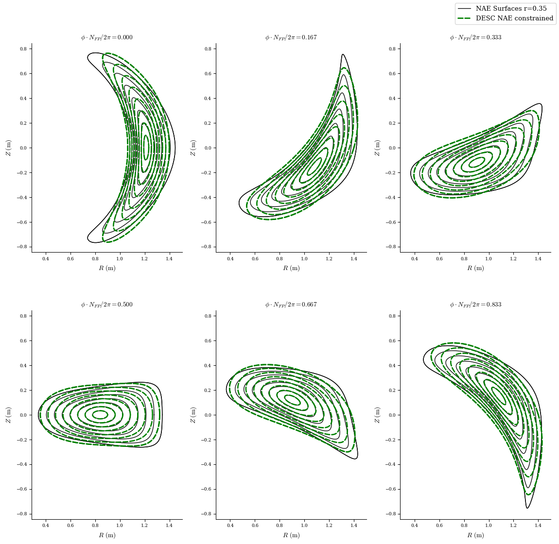
Again we can plot the surfaces, and we see that in this case, the near axis behavior is preserved, while the outer surfaces differ. This is expected, as the NAE from QSC is only valid asymptotically near the axis. By constraining this behavior we are able to keep all the desireable properties of the NAE where they are valid without overly constraining the problem.
[11]:
fig, ax = plot_comparison(
eqs=[eq_fit, eq_NAE],
labels=[f"NAE Surfaces r={r}", f"DESC NAE constrained"],
color=["k", "g"],
ls=["-", "--"],
figsize=(12, 12),
theta=0,
lw=[1, 2],
)
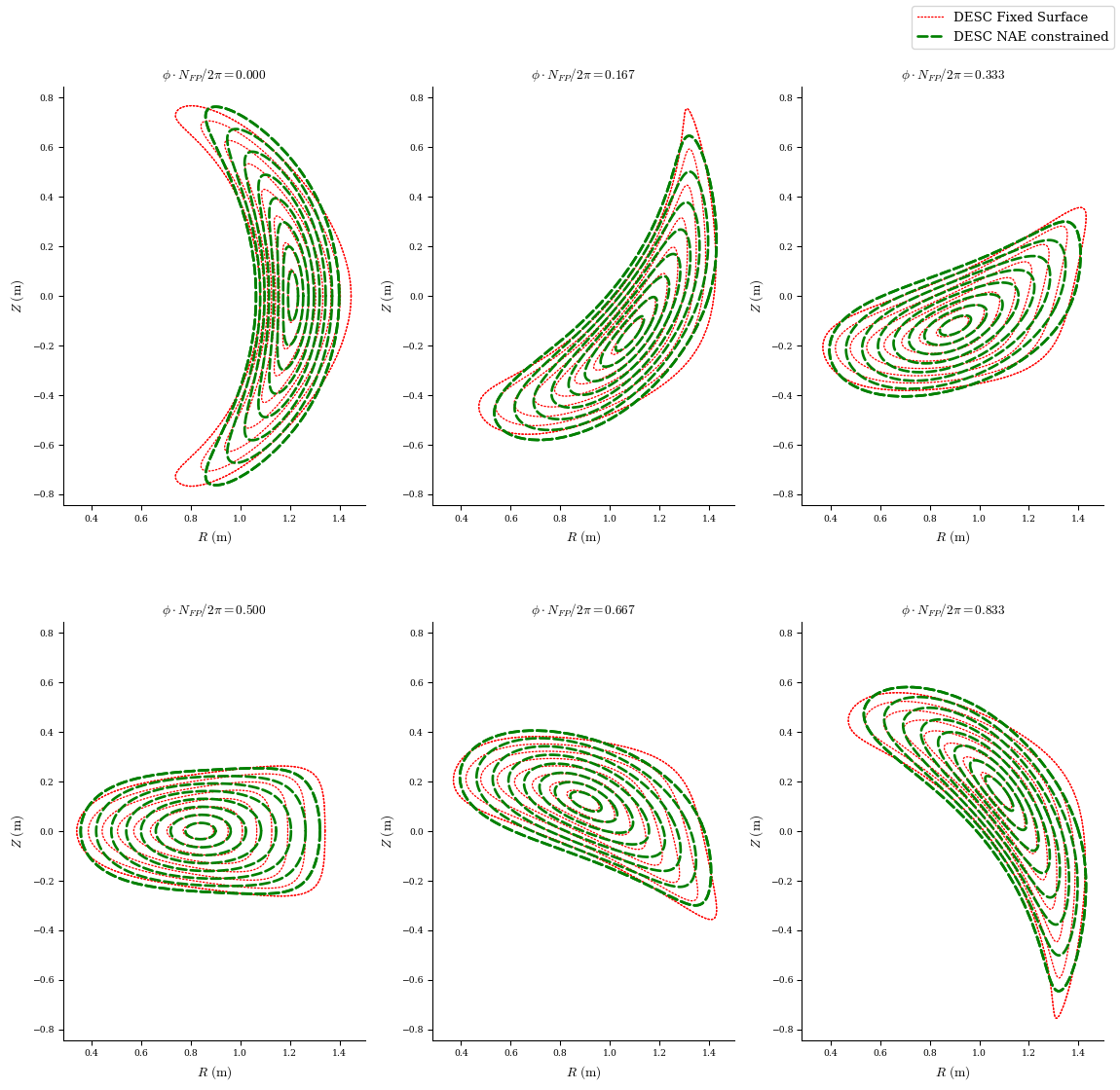
fig, ax = plot_comparison(
eqs=[eq_fixed_bdry, eq_NAE],
labels=[f"DESC Fixed Surface", f"DESC NAE constrained"],
color=["r", "g"],
ls=[":", "--"],
figsize=(12, 12),
theta=0,
lw=[1, 2],
);
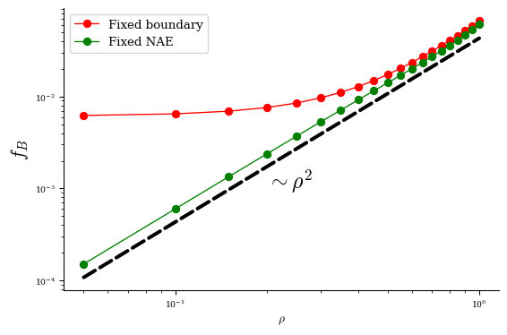
As a final comparison, we can plot the QS error for the fixed boundary and fixed NAE solves. We see that by fixing the NAE behavior, we are able to preserve the QS from the original QSC equilibrium, with the expected scaling in QS error going as \(\rho^2\).
[12]:
fix, ax = plt.subplots()
plot_qs_error(
    eq_fixed_bdry,
    fC=False,
    fT=False,
    log=True,
    ax=ax,
    color=["r"],
    legend=False,
    labels=["Fixed boundary"],
    figsize=(8, 8),
)
fig, ax, dataQS = plot_qs_error(
    eq_NAE,
    fC=False,
    fT=False,
    log=True,
    ax=ax,
    color=["g"],
    legend=False,
    labels=["Fixed NAE"],
    return_data=True,
)

ax.legend()
ax.set_xscale("log")
ax.set_yscale("log")

ax.plot(
    dataQS["rho"],
    dataQS["rho"] ** 2 * (np.max(dataQS["f_B"]) * 0.7),
    "k--",
    lw=3,
)
ax.text(0.2, 1e-3, r"$\sim \rho^2$", size=18)
ax.set_ylabel("$f_B$", fontsize=16);
# f_B = sqrt(sum(symmetry-breaking modes**2)) / sqrt(sum(all modes**2))
The correct behaviour near the axis may be also checked by assessing directly other features of the equilibrium; most notably, the behaviour of |B| on axis, the rotational transform on axis, as well as the form of \(\lambda\). Starting from the rotational transform, we may compare the values obtained in the equilibrium to those of the near-axis expansion.
[13]:
import matplotlib.pyplot as plt
from desc.plotting import plot_fsa

rho = np.linspace(0, 1e-1)
fig, ax, iota_nae = plot_fsa(
    eq_NAE, "iota", rho=rho, return_data=True, lw=6, linecolor="g"
)
fig, ax, iota_surf = plot_fsa(
    eq_fixed_bdry, "iota", rho=rho, ax=ax, return_data=True, linecolor="r", lw=3
)
plt.plot(rho, np.ones(np.size(rho)) * qsc_eq.iota, linestyle="--", lw=3, c="b")
plt.legend(["Fixed NAE", "Fixed boundary", "NAE"])
print(
    "Relative error in the rotational transform (fixed NAE): ",
    (iota_nae["iota"][0] - qsc_eq.iota) / qsc_eq.iota,
)
print(
    "Relative error in the rotational transform (fixed surface): ",
    (iota_surf["iota"][0] - qsc_eq.iota) / qsc_eq.iota,
)
/CODES/DESC/desc/utils.py:520: FutureWarning: argument linecolor has been renamed to color, linecolor will be removed in a future release
  warnings.warn(
/CODES/DESC/desc/utils.py:520: FutureWarning: argument linecolor has been renamed to color, linecolor will be removed in a future release
  warnings.warn(
Relative error in the rotational transform (fixed NAE):  -0.00047958376645073107
Relative error in the rotational transform (fixed surface):  0.09045094033839847
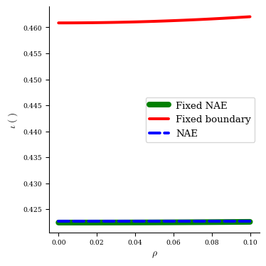
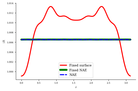
This clearly shows that the constraint is working as it is intended. A similar expected behaviour can be found for other features of the equilibrium such as the magnetic field on axis.
[14]:
from desc.compute import data_index
from desc.grid import LinearGrid

grid = LinearGrid(theta=np.array(0.0), N=100, NFP=eq_fixed_bdry.NFP, rho=np.array(0.0))
# Evaluate B modes near the axis
data_surf = eq_fixed_bdry.compute(["|B|"], grid=grid)
data_nae = eq_NAE.compute(["|B|"], grid=grid)
phi = grid.nodes[:, 2]

plt.plot(phi, data_surf["|B|"], lw=3, c="r")
plt.plot(phi, data_nae["|B|"], lw=6, c="g")
plt.plot(phi, np.ones(np.size(phi)) * qsc_eq.B0, linestyle="--", lw=3, c="b")
plt.xlabel("$\\phi$")
plt.ylabel("$|B|$")
plt.legend(["Fixed surface", "Fixed NAE", "NAE"])
plt.show()
Finally, we may check \(\lambda\) on axis and compare it to \(\nu\) from within the near-axis expansion.
\(\lambda\) is the poloidal stream function used in DESC which transforms the computational poloidal angle \(\theta\) into the straight-field-line (SFL) poloidal angle \(\theta_{PEST} = \theta + \lambda\) (So B is “straight” when plotted in this poloidal angle and the cylindrical toroidal angle \(\phi\)).
Now, the NAE describes flux surfaces using the Boozer poloidal angle \(\theta_B\), and we are constraining our solution to be asymptotically equivalent to the NAE, so our computational poloidal angle on-axis should approach \(\theta = \theta_B\).
We also know that \(\theta_{PEST} = \theta_B - \iota \nu\) where \(\nu = \phi_B - \phi\), with \(\phi_B\) being the Boozer toroidal angle.
Taken together with \(\theta_{PEST} = \theta + \lambda\), we find that on-axis we expect our DESC NAE-constrained solution to have \(\lambda = -\iota \nu\), where \(\nu\) is known already from the NAE.
[15]:
# Evaluate lambda at the axis
data_surf = eq_fixed_bdry.compute("lambda", grid=grid)
data_nae = eq_NAE.compute("lambda", grid=grid)
lam_surf = data_surf["lambda"]
lam_nae = data_nae["lambda"]

print(
    "Deviation of theta from Boozer angle (fixed surface)",
    np.mean(np.abs(lam_surf + qsc_eq.iota * qsc_eq.nu_spline(phi))),
)
print(
    "Deviation of theta from Boozer angle (fixed nae)",
    np.mean(np.abs(lam_nae + qsc_eq.iota * qsc_eq.nu_spline(phi))),
)
plt.plot(phi, lam_surf, lw=3, c="r")
plt.plot(phi, lam_nae, lw=6, c="g")
plt.plot(phi, -qsc_eq.iota * qsc_eq.nu_spline(phi), linestyle="--", lw=3, c="b")
plt.xlabel("$\\phi$")
plt.ylabel("$\\lambda$")
plt.legend(["Fixed surface", "Fixed NAE", "NAE"])
plt.show()
Deviation of theta from Boozer angle (fixed surface) 0.10325454992645072
Deviation of theta from Boozer angle (fixed nae) 0.0053119893702406355
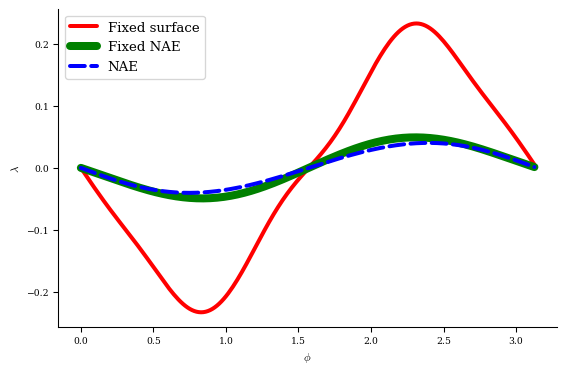
The above comparison shows that the DESC equilibrium constructed with the near-axis constraint is consistent with the near-axis behaviour.