Advanced Equilibrium & Continuation
[1]:
import sys
import os

sys.path.insert(0, os.path.abspath("."))
sys.path.append(os.path.abspath("../../../"))
In this example, we will discuss manually selecting the steps in a continuation method for solving an equilibrium.
Running DESC On HELIOTRON Example Case
We could run a HELIOTRON case from a DESC input file directly, but let’s first see how to convert a VMEC input file to a DESC input file.
In this directory is an input.HELIOTRON VMEC file which contains a 19 field-period, finite beta HELIOTRON fixed boundary stellarator. To convert the input, we simply run DESC from the command line with
python -m desc -vv input.HELIOTRON -o input.HELIOTRON_output.h5.
You can leave out python -m if you’ve added DESC to your python path. The -vv flag is for double verbosity. The -o flag specifies the filename of the output HDF5 file (XXX_output.h5 by default). See the command line docs for more information.
The conversion creates a new file with _desc appended to the file name. The above command automatically converts the VMEC input file to a DESC input file and begins solving it. There are many DESC solver options without VMEC analogs, such as the multi-grid continuation method steps, so DESC will automatically choose a conservative continuation method when ran in this way, which is generally recommended for most equilibria to ensure robust convergence.
Generally, the most important parameters to tweak are related to the spectral resolution and the continuation method. DESC leverages a multi-grid continuation method to allow for robust convergence of highly shaped equilibria. The following parameters control this method:
Spectral Resolution
L_rad(int): Maximum radial mode number for the Fourier-Zernike basis.default =
M_polifspectral_indexing = ANSIdefault =
2*M_polifspectral_indexing = FringeFor more information see Basis functions and collocation nodes.
M_pol(int): Maximum poloidal mode number for the Fourier-Zernike basis. Required input.N_tor(int): Maximum toroidal mode number for the Fourier-Zernike basis.default = 0
L_grid(int): Radial resolution of nodes in collocation grid.default =
M_gridifspectral_indexing = ANSIdefault =
2*M_gridifspectral_indexing = Fringe
M_grid(int): Poloidal resolution of nodes in collocation grid.default =
2*M_pol
N_grid(int): Toroidal resolution of nodes in collocation grid.default =
2*N_tor
When M_grid = M_pol, the number of collocation nodes in each toroidal cross-section is equal to the number of Zernike polynomials in a FourierZernike basis set of the samel resolution L_rad = M_pol. When N_grid = N_tor, the number of nodes with unique toroidal angles is equal to the number of terms in the toroidal Fourier series. Convergence is typically superior when the number of nodes exceeds the number of spectral coefficients, so by default the collocation grids are oversampled
with respect to the spectral resolutions.
It is recommended to NOT include anything for the pres_ratio or bdry_ratio arguments, as then a conservative, automated multi-grid method will be used that has been found to be very robust. If you want to instead control the multi-grid steps manually, these arguments can also be passed as arrays, where each element denotes the value to use at that iteration. Array elements are delimited by either a space, comma ,, or semicolon ;. Arrays can also be created using the shorthand
notation start:interval:end and (value)x(repititions). For example, an input line of M_pol = 6:2:10, 10; 11x2 12 is equivalent to M_pol = 6, 8, 10, 10, 11, 11, 12.
Continuation Method
pres_ratio(float): Multiplier on the pressure profile. Default =1.0.bdry_ratio(float): Multiplier on the 3D boundary modes. Default =1.0.pert_order(int): Order of the perturbation approximation:0= no perturbation,1= linear,2= quadratic,3= cubic. Default =2.
When pres_ratio = 1 and bdry_ratio = 1, the equilibrium is solved using the exact boundary modes and pressure profile as input. pres_ratio = 0 assumes a vanishing beta pressure profile. bdry_ratio = 0 ignores all the non-axisymmetric boundary modes (reducing the input to a tokamak).
Again, it is recommended to only pass in a single argument for these parameters (the final pressure or boundary ratio for pres_ratio and bdry_ratio, and the desired pert_order), which will then cause the automated multi-grid continuation method to be used, which has the greatest robustness. These arguments can also be passed as arrays for each iteration, with the same notation as the other continuation parameters. This example will start by solving a vacuum tokamak, then perturb the
pressure profile to solve a finite-beta tokamak, and finally perturb the boundary to solve the finite-beta stellarator. If only one value is given, as with pert_order in this example, that value will be used for all iterations.
In general, we can design an input to use a 3-step continuation method:
Solve a zero beta (
pres_ratio=0) axisymmetric tokamak (bdry_ratio=0), which will use only the axisymmetric modes of the boundary. Let’s choose a radial and poloidal resolution ofL_rad=6andM_pol=6, and since it is axisymmetric we can use no toroidal resolution:N_tor=0. We’ll also choose collocation grid resolutions that are twice our spectral resolutions:L_grid=12,M_grid=12,N_grid=0.Solve a finite-beta tokamak (
pres_ratio=1) and increase our radial and poloidal resolutions:L_rad=8,M_pol=8,N_tor=0and the corresponding grid resolutions:L_grid=16,M_grid=16,N_grid=0.Add in the non-axisymmetric modes and solve the full stellarator by setting
bdry_ratio=1and adding toroidal resolution:N_tor=3,N_grid=6.
As a visual, these modifications would change the input file below to the one following it.
Without 3-step continuation method
# global parameters
sym = 1
NFP = 19
Psi = 1.0

# spectral resolution
L_rad = 8
M_pol = 8
N_tor = 3
L_grid = 16
M_grid = 16
N_grid = 6

# continuation parameters
bdry_ratio = 1
pres_ratio = 1
pert_order = 1

# solver tolerances
ftol = 1e-2
xtol = 1e-6
gtol = 1e-6
nfev = 0

# solver methods
optimizer = lsq-exact
objective = force
bdry_mode = lcfs
spectral_indexing = ansi

# pressure and rotational transform/current profiles
l:   0  p =   1.80000000E+04    i =   1.00000000E+00
l:   2  p =  -3.60000000E+04    i =   1.50000000E+00
l:   4  p =   1.80000000E+04    i =   0.00000000E+00

# fixed-boundary surface shape
l:   0  m:   0  n:   0  R1 =   1.00000000E+01   Z1 =   0.00000000E+00
l:   0  m:   1  n:   0  R1 =  -1.00000000E+00   Z1 =   0.00000000E+00
l:   0  m:   0  n:   1  R1 =   0.00000000E+00   Z1 =   0.00000000E+00
l:   0  m:   1  n:   1  R1 =  -3.00000000E-01   Z1 =   0.00000000E+00
l:   0  m:  -1  n:  -1  R1 =   3.00000000E-01   Z1 =   0.00000000E+00
l:   0  m:  -1  n:   0  R1 =   0.00000000E+00   Z1 =   1.00000000E+00
l:   0  m:   0  n:  -1  R1 =   0.00000000E+00   Z1 =   0.00000000E+00
l:   0  m:  -1  n:   1  R1 =   0.00000000E+00   Z1 =  -3.00000000E-01
l:   0  m:   1  n:  -1  R1 =   0.00000000E+00   Z1 =  -3.00000000E-01

# magnetic axis initial guess
n:   0  R0 =   1.00000000E+01   Z0 =   0.00000000E+00
With 3-step continuation method
# global parameters
sym = 1
NFP = 19
Psi = 1.0

# spectral resolution
L_rad =   6,  8
M_pol =   6,  8
N_tor =   0,  0, 3
L_grid = 12, 16
M_grid = 12, 16
N_grid =  0,  0, 6

# continuation parameters
bdry_ratio = 0, 0, 1
pres_ratio = 0, 1
pert_order = 1

# solver tolerances
ftol = 1e-2
xtol = 1e-6
gtol = 1e-6
nfev = 0

# solver methods
optimizer = lsq-exact
objective = force
bdry_mode = lcfs
spectral_indexing = ansi

# pressure and rotational transform/current profiles
l:   0  p =   1.80000000E+04    i =   1.00000000E+00
l:   2  p =  -3.60000000E+04    i =   1.50000000E+00
l:   4  p =   1.80000000E+04    i =   0.00000000E+00

# fixed-boundary surface shape
l:   0  m:   0  n:   0  R1 =   1.00000000E+01   Z1 =   0.00000000E+00
l:   0  m:   1  n:   0  R1 =  -1.00000000E+00   Z1 =   0.00000000E+00
l:   0  m:   0  n:   1  R1 =   0.00000000E+00   Z1 =   0.00000000E+00
l:   0  m:   1  n:   1  R1 =  -3.00000000E-01   Z1 =   0.00000000E+00
l:   0  m:  -1  n:  -1  R1 =   3.00000000E-01   Z1 =   0.00000000E+00
l:   0  m:  -1  n:   0  R1 =   0.00000000E+00   Z1 =   1.00000000E+00
l:   0  m:   0  n:  -1  R1 =   0.00000000E+00   Z1 =   0.00000000E+00
l:   0  m:  -1  n:   1  R1 =   0.00000000E+00   Z1 =  -3.00000000E-01
l:   0  m:   1  n:  -1  R1 =   0.00000000E+00   Z1 =  -3.00000000E-01

# magnetic axis initial guess
n:   0  R0 =   1.00000000E+01   Z0 =   0.00000000E+00
Auto generated input
When automatically converting the VMEC input file, DESC only lists the desired final resolutions, which then will trigger the automatic multi-grid continuation method, which is conservative but very robust.
# This DESC input file was auto generated from the VMEC input file
# /DESC/docs/notebooks/tutorials/input.HELIOTRON
# For details on the various options see https://desc-docs.readthedocs.io/en/stable/input.html

# global parameters
sym = 1
NFP =  19
Psi = 1.00000000

# spectral resolution
L_rad = 8
M_pol = 8
N_tor = 3
L_grid = 16
M_grid = 16
N_grid = 6

# continuation parameters
pert_order = 2.0

# solver tolerances

# solver methods
optimizer = lsq-exact
objective = force
bdry_mode = lcfs
spectral_indexing = ansi

# pressure and rotational transform/current profiles
l:   0  p =   1.80000000E+04    i =   1.00000000E+00
l:   2  p =  -3.60000000E+04    i =   1.50000000E+00
l:   4  p =   1.80000000E+04    i =   0.00000000E+00

# fixed-boundary surface shape
l:   0  m:  -1  n:  -1  R1 =   3.00000000E-01   Z1 =   0.00000000E+00
l:   0  m:  -1  n:   0  R1 =   0.00000000E+00   Z1 =   1.00000000E+00
l:   0  m:  -1  n:   1  R1 =   0.00000000E+00   Z1 =  -3.00000000E-01
l:   0  m:   0  n:  -1  R1 =   0.00000000E+00   Z1 =   0.00000000E+00
l:   0  m:   0  n:   0  R1 =   1.00000000E+01   Z1 =   0.00000000E+00
l:   0  m:   0  n:   1  R1 =   0.00000000E+00   Z1 =   0.00000000E+00
l:   0  m:   1  n:  -1  R1 =   0.00000000E+00   Z1 =  -3.00000000E-01
l:   0  m:   1  n:   0  R1 =  -1.00000000E+00   Z1 =   0.00000000E+00
l:   0  m:   1  n:   1  R1 =  -3.00000000E-01   Z1 =   0.00000000E+00

# magnetic axis initial guess
n:   0  R0 =   1.00000000E+01   Z0 =   0.00000000E+00
Loading the results
DESC provides utility functions to load and compare equilibria. These will be covered in detail later in the tutorial. For now, notice that DESC saves solutions as EquilibriaFamily objects. An EquilibriaFamily is essentially a list of equilibria, which can be indexed to retrieve individual equilibria. Higher indices hold equilibria solved later in the continuation process. You can retrieve the final state of a DESC equilibrium solve with eq = desc.io.load("XXX_output.h5")[-1].
[3]:
%matplotlib inline
import desc
from desc.plotting import plot_comparison, plot_section
[4]:
eq_fam = desc.io.load("input.HELIOTRON_output.h5")
print("Number of equilibria in the EquilibriaFamily:", len(eq_fam))
fig, ax = plot_comparison(
    eqs=[eq_fam[1], eq_fam[3], eq_fam[-1]],
    labels=[
        "Axisymmetric w/o pressure",
        "Axisymmetric w/ pressure",
        "Nonaxisymmetric w/ pressure",
    ],
)
Number of equilibria in the EquilibriaFamily: 8
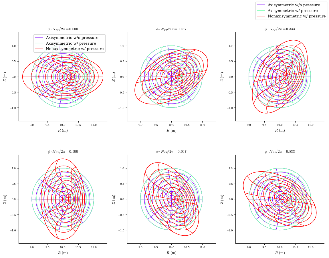
Let’s continue the tutorial by comparing the final equilibria that result from the
first input file which lacks a continuation method
last input file which was auto generated by DESC
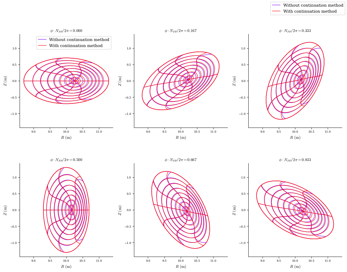
Flux surface comparison
[5]:
eq_fam_no_continuation = desc.io.load("input.HELIOTRON_desc_no_continuation_output.h5")

plot_comparison(
    eqs=[eq_fam_no_continuation[-1], eq_fam[-1]],
    labels=["Without continuation method", "With continuation method"],
);
Force error comparison
[6]:
f1 = (
    eq_fam_no_continuation[-1].compute("<|F|>_vol")["<|F|>_vol"]
    / eq_fam_no_continuation[-1].compute("<|grad(|B|^2)|/2mu0>_vol")[
        "<|grad(|B|^2)|/2mu0>_vol"
    ]
)
f2 = (
    eq_fam[-1].compute("<|F|>_vol")["<|F|>_vol"]
    / eq_fam[-1].compute("<|grad(|B|^2)|/2mu0>_vol")["<|grad(|B|^2)|/2mu0>_vol"]
)
print(f"Force error without continuation: {f1:.4e}")
print(f"Force error with continuation: {f2:.4e}")
Force error without continuation: 9.3711e-03
Force error with continuation: 7.3832e-03
Analysis
While the continuation method took a bit longer to run, it yielded a solution with slightly lower normalized force error across the volume as compared to the solution without the continuation method. For strongly shaped equilibria, using the continuation method usually gives significantly better solutions in less time, as well as being extremely robust.
The force error is still relatively high, this is because we are using a relatively low resolution just to showcase the code functionality. The force error decreases when solved with higher resolution.
For a more realistic example of using the continuation method to solve a complicated equilibrium, see the NCSX example input file.