Basic Equilibrium

DESC is a 3D MHD equilibrium and optimization code suite, which solves the ideal MHD equilibrium equations to find stellarator equilibria.

Like VMEC, DESC requires 4 main inputs to define the equilibrium problem:

Pressure Profile
Rotational Transform or Toroidal Current Profile
Last Closed Flux Surface Boundary Shape
Total toroidal magnetic flux enclosed by the LCFS

DESC can be run both with a text input file from the command line (e.g. python -m desc INPUT_FILE) or through python scripts (which offers more options than the text file for equilibrium solving and optimization). This tutorial notebook will focus on basic functionality for solving an equilibrium.

Installing DESC

The installation instructions are located in the installation documentation page.

Once these instructions are followed and DESC is installed correctly, you should be able to import a module from desc such as desc.io without any errors.

[1]:

import sys
import os

sys.path.insert(0, os.path.abspath("."))
sys.path.append(os.path.abspath("../../../"))

[2]:

import desc.io

DESC version 0.10.2+349.g81f43916.dirty,using JAX backend, jax version=0.4.13, jaxlib version=0.4.13, dtype=float64
Using device: CPU, with 3.46 GB available memory

Running DESC from a VMEC input

Perhaps the simplest way to run DESC if you already have a VMEC input file for your equilibrium is to simply pass that to DESC on the command line.

In this directory is an input.HELIOTRON VMEC file which contains a 19 field-period, finite beta HELIOTRON fixed boundary stellarator. To convert the input, we simply run DESC from the command line with

python -m desc -vv input.HELIOTRON -o input.HELIOTRON_output.h5.

You can leave out python -m if you’ve added DESC to your python path. The -vv flag is for double verbosity. The -o flag specifies the filename of the output HDF5 file (XXX_output.h5 by default). See the command line docs for more information.

The conversion creates a new file with _desc appended to the file name. The above command automatically converts the VMEC input file to a DESC input file and begins solving it. There are many DESC solver options without VMEC analogs, such as the multi-grid continuation method steps, so DESC will automatically choose a conservative continuation method when ran in this way, which is generally recommended for most equilibria to ensure robust convergence.

Generally, the most important parameters to tweak are related to the spectral resolution and the continuation method. DESC leverages a multi-grid continuation method to allow for robust convergence of highly shaped equilibria. The following parameters control this method:

Spectral Resolution

L_rad (int): Maximum radial mode number for the Fourier-Zernike basis.
- default = M_pol if spectral_indexing = ANSI
- default = 2*M_pol if spectral_indexing = Fringe
- For more information see Basis functions and collocation nodes.
M_pol (int): Maximum poloidal mode number for the Fourier-Zernike basis. Required input.
N_tor (int): Maximum toroidal mode number for the Fourier-Zernike basis.
- default = 0
L_grid (int): Radial resolution of nodes in collocation grid.
- default = M_grid if spectral_indexing = ANSI
- default = 2*M_grid if spectral_indexing = Fringe
M_grid (int): Poloidal resolution of nodes in collocation grid.
- default = 2*M_pol
N_grid (int): Toroidal resolution of nodes in collocation grid.
- default = 2*N_tor

When M_grid = M_pol, the number of collocation nodes in each toroidal cross-section is equal to the number of Zernike polynomials in a FourierZernike basis set of the same resolution L_rad = M_pol. When N_grid = N_tor, the number of nodes with unique toroidal angles is equal to the number of terms in the toroidal Fourier series. Convergence is typically superior when the number of nodes exceeds the number of spectral coefficients, so by default the collocation grids are oversampled with respect to the spectral resolutions.

Loading the results

DESC provides utility functions to load and compare equilibria. These will be covered in detail later in the tutorial. For now, notice that DESC saves solutions as EquilibriaFamily objects. An EquilibriaFamily is essentially a list of equilibria, which can be indexed to retrieve individual equilibria. Higher indices hold equilibria solved later in the continuation process. You can retrieve the final state of a DESC equilibrium solve with eq = desc.io.load("XXX_output.h5")[-1].

[3]:

%matplotlib inline
from desc.plotting import plot_comparison, plot_section

[4]:

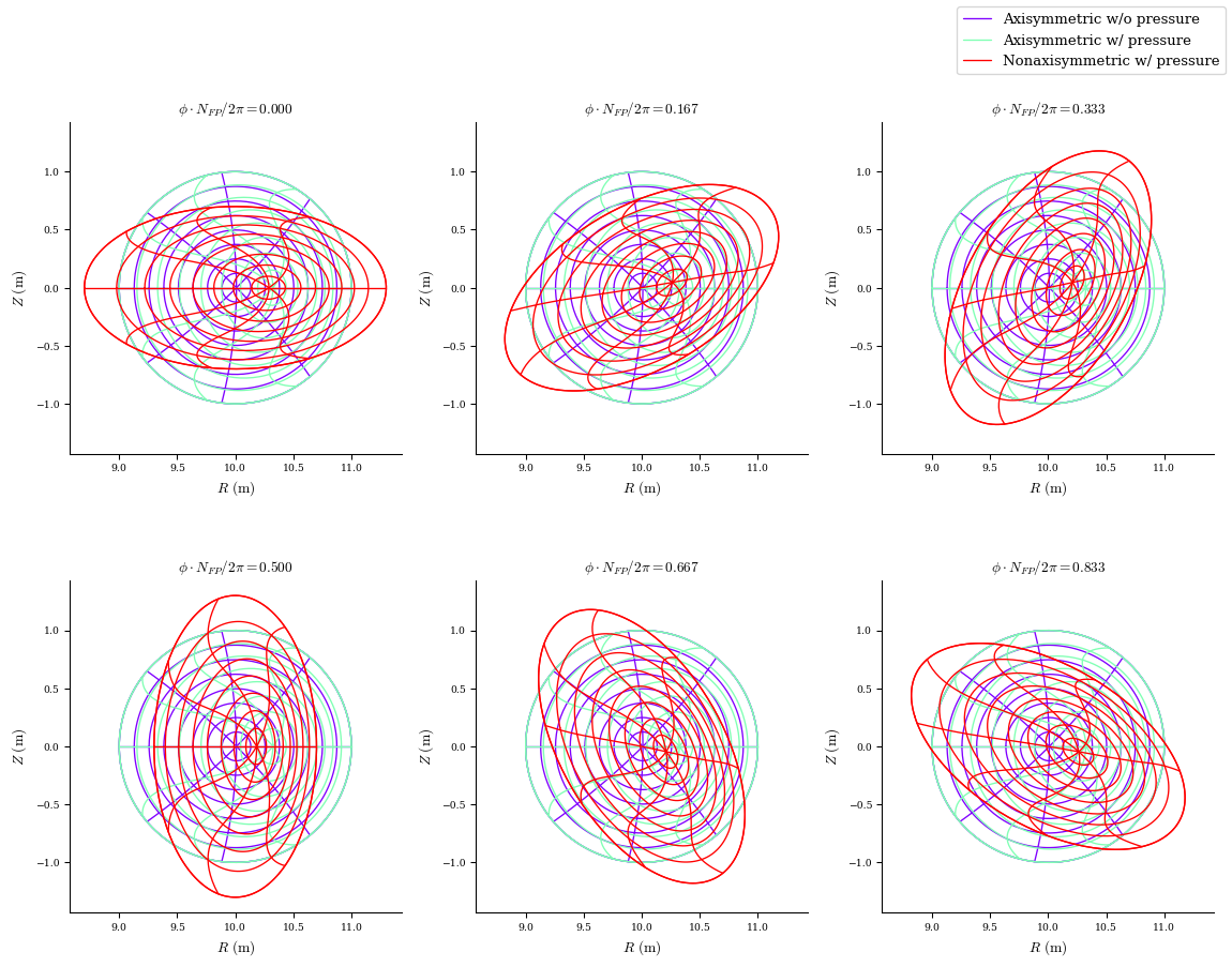
eq_fam = desc.io.load("input.HELIOTRON_output.h5")
print("Number of equilibria in the EquilibriaFamily:", len(eq_fam))
fig, ax = plot_comparison(
    eqs=[eq_fam[1], eq_fam[3], eq_fam[-1]],
    labels=[
        "Axisymmetric w/o pressure",
        "Axisymmetric w/ pressure",
        "Nonaxisymmetric w/ pressure",
    ],
)

Number of equilibria in the EquilibriaFamily: 8

../../_images/notebooks_tutorials_basic_equilibrium_10_1.png

Creating an Equilibrium from scratch

The recommended way to work with DESC is through python scripts, in which we construct and solve an Equilibrium object.

We initialize the Equilibrium with the desired resolution, and the inputs specified above: - Boundary shape, as a FourierRZToroidalSurface - Profiles, as Profile objects (there are several different options, the most common is PowerSeriesProfile) - Total flux Psi as a float

[5]:

from desc.equilibrium import Equilibrium
from desc.geometry import FourierRZToroidalSurface
from desc.profiles import PowerSeriesProfile

To start, we can use the same boundary surface as before, extracting it from the VMEC input file with FourierRZToroidalSurface.from_input_file:

[6]:

surf1 = FourierRZToroidalSurface.from_input_file("input.HELIOTRON")

Alternatively, we could construct the surface by specifying the Fourier coefficients and mode numbers manually.

The boundary is represented by a double Fourier series for R and Z in terms of a poloidal angle \(\theta\) and the geometric toroidal angle \(\zeta\). We specify the mode numbers for R and Z as 2D arrays of [m,n] pairs, and the coefficients as a 1D array.

In DESC the double Fourier series for R and Z are defined in a slightly different manner than VMEC:

\[\begin{split}\begin{align} R^b(\theta,\zeta) &= \sum^M \sum^N R^b_{mn} \mathcal{G}^{m}_{n}(\theta,\zeta)\\ Z^b(\theta,\zeta) &= \sum^M \sum^N Z^b_{mn} \mathcal{G}^{m}_{n}(\theta,\zeta) \end{align}\end{split}\]

where

\[\begin{split}\mathcal{G}^{m}_{n}(\theta,\zeta) = \begin{cases} \cos(|m|\theta)\cos(|n|N_{FP}\zeta) &\text{for }m\ge0, n\ge0 \\ \cos(|m|\theta)\sin(|n|N_{FP}\zeta) &\text{for }m\ge0, n<0 \\ \sin(|m|\theta)\cos(|n|N_{FP}\zeta) &\text{for }m<0, n\ge0 \\ \sin(|m|\theta)\sin(|n|N_{FP}\zeta) &\text{for }m<0, n<0. \end{cases}\end{split}\]

Note: in DESC, radial modes are indexed by l, poloidal modes by m, and toroidal modes by n

[7]:

surf2 = FourierRZToroidalSurface(
    R_lmn=[10.0, -1.0, -0.3, 0.3],
    modes_R=[
        (0, 0),
        (1, 0),
        (1, 1),
        (-1, -1),
    ],  # (m,n) pairs corresponding to R_mn on previous line
    Z_lmn=[1, -0.3, -0.3],
    modes_Z=[(-1, 0), (-1, 1), (1, -1)],
    NFP=19,
)

For profiles, we will use the standard PowerSeriesProfile which represents a function as a power series in the radial coordinate \(\rho\) which is the square root of the normalized toroidal flux: \(\rho = \sqrt{\Psi/\Psi_b}\) (Note this is different from VMEC which uses the normalized toroidal flux without the square root). We could also use splines (SplineProfile), or Zernike polynomials (FourierZernikeProfile), for more options, see the `desc.profiles module <https://desc-docs.readthedocs.io/en/stable/api.html#profiles>`__

[8]:

pressure = PowerSeriesProfile(
    [1.8e4, 0, -3.6e4, 0, 1.8e4]
)  # coefficients in ascending powers of rho
iota = PowerSeriesProfile([1, 0, 1.5])  # 1 + 1.5 r^2

Finally, we create the equilibrium using the objects we just made, leaving the other parameters at their defaults. The number of field periods by default is inferred from the given surface.

[9]:

eq = Equilibrium(
    L=8,  # radial resolution
    M=8,  # poloidal resolution
    N=3,  # toroidal resolution
    surface=surf1,
    pressure=pressure,
    iota=iota,
    Psi=1.0,  # total flux, in Webers
)

We now have an Equilibrium object, but it is generally not actually in equilibrium, as the default initial guess is just to scale the outermost flux surface.

To find the actual solution, we must solve the equilibrium. There are two primary ways to do this in DESC:

eq.solve is a method of the Equilibrium class that is best used when starting close to the correct solution, or for refining a solution after optimization, for example. Generally not recommended for “cold start” solves.
desc.continuation.solve_continuation_automatic uses a multi-grid continuation method to arrive at a particular desired equilibrium. It is generally very robust, and is the recommended method.

Here, we will use both methods

[10]:

eq1, info = eq.solve(verbose=3, copy=True)

Building objective: force
Precomputing transforms
Timer: Precomputing transforms = 2.13 sec
Timer: Objective build = 4.88 sec
Timer: Linear constraint projection build = 9.24 sec
Compiling objective function and derivatives: ['force']
Timer: Objective compilation time = 3.31 sec
Timer: Jacobian compilation time = 7.61 sec
Timer: Total compilation time = 10.9 sec
Number of parameters: 351
Number of objectives: 2106
Starting optimization
Using method: lsq-exact
   Iteration     Total nfev        Cost      Cost reduction    Step norm     Optimality
       0              1          2.052e-01                                    8.741e+00
       1              2          1.713e-02      1.880e-01      2.539e-01      3.113e+00
       2              3          1.289e-03      1.584e-02      3.003e-01      4.235e-01
       3              4          9.287e-04      3.600e-04      1.775e-01      1.376e+00
       4              5          1.895e-04      7.392e-04      1.178e-01      4.320e-01
       5              6          3.929e-05      1.502e-04      7.147e-02      1.531e-01
       6              7          2.165e-05      1.764e-05      3.119e-02      2.926e-02
       7              8          2.115e-05      5.045e-07      1.633e-02      1.893e-02
       8              9          2.089e-05      2.550e-07      1.821e-02      7.787e-03
       9             10          2.082e-05      7.414e-08      1.102e-02      7.625e-03
Optimization terminated successfully.
`ftol` condition satisfied.
         Current function value: 2.082e-05
         Total delta_x: 6.849e-01
         Iterations: 9
         Function evaluations: 10
         Jacobian evaluations: 10
Timer: Solution time = 18.4 sec
Timer: Avg time per step = 1.84 sec
Start of solver
Total (sum of squares):  2.052e-01,
Maximum absolute Force error:  1.584e+06 (N)
Minimum absolute Force error:  2.242e+01 (N)
Average absolute Force error:  2.478e+05 (N)
Maximum absolute Force error:  6.052e-02 (normalized)
Minimum absolute Force error:  8.563e-07 (normalized)
Average absolute Force error:  9.465e-03 (normalized)
R boundary error:  0.000e+00 (m)
Z boundary error:  0.000e+00 (m)
Fixed-Psi error:  0.000e+00 (Wb)
Fixed-pressure profile error:  0.000e+00 (Pa)
Fixed-iota profile error:  0.000e+00 (dimensionless)
End of solver
Total (sum of squares):  2.082e-05,
Maximum absolute Force error:  5.903e+04 (N)
Minimum absolute Force error:  1.145e+00 (N)
Average absolute Force error:  2.314e+03 (N)
Maximum absolute Force error:  2.255e-03 (normalized)
Minimum absolute Force error:  4.374e-08 (normalized)
Average absolute Force error:  8.838e-05 (normalized)
R boundary error:  0.000e+00 (m)
Z boundary error:  0.000e+00 (m)
Fixed-Psi error:  0.000e+00 (Wb)
Fixed-pressure profile error:  0.000e+00 (Pa)
Fixed-iota profile error:  0.000e+00 (dimensionless)

[11]:

from desc.continuation import solve_continuation_automatic

eqf = solve_continuation_automatic(eq.copy(), verbose=3)

================
Step 1
================
Spectral indexing: ansi
Spectral resolution (L,M,N)=(6,6,0)
Node resolution (L,M,N)=(12,12,0)
Boundary ratio = 0
Pressure ratio = 0
Perturbation Order = 2
Objective: force
Optimizer: lsq-exact
================
Building objective: force
Precomputing transforms
Timer: Precomputing transforms = 3.92 sec
Timer: Objective build = 5.22 sec
Timer: Linear constraint projection build = 5.09 sec
Compiling objective function and derivatives: ['force']
Timer: Objective compilation time = 1.50 sec
Timer: Jacobian compilation time = 3.06 sec
Timer: Total compilation time = 4.57 sec
Number of parameters: 27
Number of objectives: 98
Starting optimization
Using method: lsq-exact
   Iteration     Total nfev        Cost      Cost reduction    Step norm     Optimality
       0              1          3.412e-03                                    5.848e-01
       1              2          1.198e-03      2.214e-03      2.956e-01      1.548e-01
       2              3          9.494e-05      1.103e-03      1.389e-01      3.834e-02
       3              4          3.942e-06      9.099e-05      2.667e-02      5.640e-03
       4              5          2.288e-07      3.713e-06      1.331e-02      9.524e-04
       5              6          3.081e-08      1.980e-07      4.450e-03      1.179e-04
       6              7          2.314e-08      7.675e-09      4.940e-03      1.317e-04
       7              8          2.171e-08      1.429e-09      4.969e-03      2.475e-05
       8              9          2.154e-08      1.705e-10      9.957e-04      3.359e-06
Optimization terminated successfully.
`ftol` condition satisfied.
         Current function value: 2.154e-08
         Total delta_x: 1.608e-01
         Iterations: 8
         Function evaluations: 9
         Jacobian evaluations: 9
Timer: Solution time = 3.86 sec
Timer: Avg time per step = 429 ms
Start of solver
Total (sum of squares):  3.412e-03,
Maximum absolute Force error:  2.067e+05 (N)
Minimum absolute Force error:  5.178e+01 (N)
Average absolute Force error:  3.277e+04 (N)
Maximum absolute Force error:  7.897e-03 (normalized)
Minimum absolute Force error:  1.978e-06 (normalized)
Average absolute Force error:  1.252e-03 (normalized)
R boundary error:  0.000e+00 (m)
Z boundary error:  0.000e+00 (m)
Fixed-Psi error:  0.000e+00 (Wb)
Fixed-pressure profile error:  0.000e+00 (Pa)
Fixed-iota profile error:  0.000e+00 (dimensionless)
End of solver
Total (sum of squares):  2.154e-08,
Maximum absolute Force error:  9.478e+02 (N)
Minimum absolute Force error:  8.292e-01 (N)
Average absolute Force error:  7.425e+01 (N)
Maximum absolute Force error:  3.621e-05 (normalized)
Minimum absolute Force error:  3.168e-08 (normalized)
Average absolute Force error:  2.836e-06 (normalized)
R boundary error:  0.000e+00 (m)
Z boundary error:  0.000e+00 (m)
Fixed-Psi error:  0.000e+00 (Wb)
Fixed-pressure profile error:  0.000e+00 (Pa)
Fixed-iota profile error:  0.000e+00 (dimensionless)
Timer: Iteration 1 total = 21.5 sec
================
Step 2
================
Spectral indexing: ansi
Spectral resolution (L,M,N)=(8,8,0)
Node resolution (L,M,N)=(16,16,0)
Boundary ratio = 0
Pressure ratio = 0
Perturbation Order = 2
Objective: force
Optimizer: lsq-exact
================
Building objective: force
Precomputing transforms
Timer: Precomputing transforms = 2.66 sec
Timer: Objective build = 3.13 sec
Timer: Linear constraint projection build = 3.80 sec
Compiling objective function and derivatives: ['force']
Timer: Objective compilation time = 1.08 sec
Timer: Jacobian compilation time = 2.55 sec
Timer: Total compilation time = 3.64 sec
Number of parameters: 48
Number of objectives: 162
Starting optimization
Using method: lsq-exact
   Iteration     Total nfev        Cost      Cost reduction    Step norm     Optimality
       0              1          2.085e-08                                    5.865e-04
       1              3          7.117e-09      1.373e-08      1.125e-02      3.934e-04
       2              4          3.080e-09      4.037e-09      1.902e-02      3.547e-04
       3              6          2.234e-10      2.857e-09      4.362e-03      1.857e-05
       4              7          1.136e-10      1.098e-10      9.103e-03      6.470e-05
       5              9          7.335e-12      1.063e-10      1.834e-03      4.481e-05
       6             11          6.772e-13      6.658e-12      6.510e-04      9.377e-06
       7             13          1.130e-13      5.642e-13      3.219e-04      2.325e-06
       8             15          6.576e-14      4.724e-14      1.611e-04      5.847e-07
       9             17          5.891e-14      6.853e-15      8.072e-05      1.475e-07
      10             19          5.717e-14      1.740e-15      4.053e-05      4.303e-08
      11             20          5.576e-14      1.409e-15      8.649e-05      3.290e-07
      12             22          5.524e-14      5.181e-16      4.738e-05      8.371e-08
Optimization terminated successfully.
`ftol` condition satisfied.
         Current function value: 5.524e-14
         Total delta_x: 4.338e-02
         Iterations: 12
         Function evaluations: 22
         Jacobian evaluations: 13
Timer: Solution time = 5.72 sec
Timer: Avg time per step = 440 ms
Start of solver
Total (sum of squares):  2.085e-08,
Maximum absolute Force error:  1.359e+03 (N)
Minimum absolute Force error:  3.405e-01 (N)
Average absolute Force error:  7.427e+01 (N)
Maximum absolute Force error:  5.192e-05 (normalized)
Minimum absolute Force error:  1.301e-08 (normalized)
Average absolute Force error:  2.837e-06 (normalized)
R boundary error:  0.000e+00 (m)
Z boundary error:  0.000e+00 (m)
Fixed-Psi error:  0.000e+00 (Wb)
Fixed-pressure profile error:  0.000e+00 (Pa)
Fixed-iota profile error:  0.000e+00 (dimensionless)
End of solver
Total (sum of squares):  5.524e-14,
Maximum absolute Force error:  1.331e+00 (N)
Minimum absolute Force error:  3.204e-03 (N)
Average absolute Force error:  1.160e-01 (N)
Maximum absolute Force error:  5.085e-08 (normalized)
Minimum absolute Force error:  1.224e-10 (normalized)
Average absolute Force error:  4.430e-09 (normalized)
R boundary error:  0.000e+00 (m)
Z boundary error:  0.000e+00 (m)
Fixed-Psi error:  0.000e+00 (Wb)
Fixed-pressure profile error:  0.000e+00 (Pa)
Fixed-iota profile error:  0.000e+00 (dimensionless)
Timer: Iteration 2 total = 22.1 sec
================
Step 3
================
Spectral indexing: ansi
Spectral resolution (L,M,N)=(8,8,0)
Node resolution (L,M,N)=(16,16,0)
Boundary ratio = 0
Pressure ratio = 0.5
Perturbation Order = 2
Objective: force
Optimizer: lsq-exact
================
Perturbing equilibrium
Building objective: force
Precomputing transforms
Timer: Precomputing transforms = 425 ms
Timer: Objective build = 750 ms
Perturbing p_l
Factorizing linear constraints
Timer: linear constraint factorize = 2.29 sec
Computing df
Timer: df computation = 8.19 sec
Factoring df
Timer: df/dx factorization = 9.59 ms
Computing d^2f
Timer: d^2f computation = 9.45 sec
||dx||/||x|| =  3.682e-02
Timer: Total perturbation = 23.1 sec
Timer: Linear constraint projection build = 544 ms
Compiling objective function and derivatives: ['force']
Timer: Objective compilation time = 1.46 sec
Timer: Jacobian compilation time = 3.10 sec
Timer: Total compilation time = 4.57 sec
Number of parameters: 48
Number of objectives: 162
Starting optimization
Using method: lsq-exact
   Iteration     Total nfev        Cost      Cost reduction    Step norm     Optimality
       0              1          5.014e-02                                    2.633e+00
       1              2          1.564e-03      4.858e-02      2.974e-01      6.573e-01
       2              4          2.503e-05      1.539e-03      7.266e-02      4.062e-02
       3              6          1.080e-05      1.422e-05      3.101e-02      1.103e-02
       4              8          8.712e-06      2.092e-06      1.193e-02      3.243e-03
       5              9          6.402e-06      2.310e-06      2.084e-02      1.434e-02
       6             11          5.065e-06      1.336e-06      1.023e-02      3.793e-03
       7             12          4.066e-06      9.994e-07      2.043e-02      1.571e-02
       8             13          3.089e-06      9.763e-07      2.095e-02      1.632e-02
       9             14          2.378e-06      7.118e-07      2.109e-02      1.679e-02
      10             15          1.892e-06      4.858e-07      2.040e-02      1.797e-02
      11             16          1.589e-06      3.026e-07      1.914e-02      1.951e-02
      12             17          1.393e-06      1.958e-07      1.811e-02      2.136e-02
      13             18          6.311e-07      7.622e-07      4.547e-03      1.351e-03
      14             19          5.966e-07      3.456e-08      8.899e-03      5.699e-03
      15             20          5.307e-07      6.588e-08      8.958e-03      5.896e-03
      16             21          4.734e-07      5.726e-08      9.104e-03      6.022e-03
      17             22          4.232e-07      5.025e-08      9.323e-03      6.101e-03
      18             23          3.789e-07      4.427e-08      9.601e-03      6.142e-03
      19             24          3.398e-07      3.912e-08      9.926e-03      6.152e-03
      20             25          3.052e-07      3.462e-08      1.029e-02      6.132e-03
      21             26          2.745e-07      3.065e-08      1.066e-02      6.085e-03
      22             27          2.474e-07      2.711e-08      1.105e-02      6.016e-03
      23             28          2.235e-07      2.392e-08      1.143e-02      5.930e-03
      24             29          2.025e-07      2.102e-08      1.178e-02      5.834e-03
      25             30          1.841e-07      1.839e-08      1.211e-02      5.736e-03
      26             31          1.681e-07      1.598e-08      1.240e-02      5.645e-03
      27             32          1.543e-07      1.379e-08      1.263e-02      5.568e-03
      28             33          1.425e-07      1.179e-08      1.282e-02      5.510e-03
      29             34          1.325e-07      9.985e-09      1.294e-02      5.477e-03
      30             35          1.242e-07      8.362e-09      1.301e-02      5.468e-03
      31             36          1.173e-07      6.918e-09      1.302e-02      5.482e-03
      32             37          9.345e-08      2.380e-08      3.343e-03      3.343e-04
      33             38          9.180e-08      1.653e-09      6.570e-03      1.363e-03
      34             39          8.914e-08      2.657e-09      6.520e-03      1.373e-03
      35             40          8.672e-08      2.419e-09      6.483e-03      1.383e-03
      36             41          8.452e-08      2.197e-09      6.444e-03      1.393e-03
      37             42          8.254e-08      1.985e-09      6.407e-03      1.403e-03
      38             43          8.076e-08      1.782e-09      6.369e-03      1.412e-03
      39             44          7.917e-08      1.587e-09      6.332e-03      1.421e-03
      40             45          7.777e-08      1.399e-09      6.295e-03      1.429e-03
      41             46          7.655e-08      1.218e-09      6.258e-03      1.438e-03
      42             47          7.551e-08      1.043e-09      6.219e-03      1.445e-03
      43             48          7.464e-08      8.739e-10      6.181e-03      1.453e-03
      44             49          7.393e-08      7.090e-10      6.141e-03      1.461e-03
Optimization terminated successfully.
`ftol` condition satisfied.
         Current function value: 7.393e-08
         Total delta_x: 2.591e-01
         Iterations: 44
         Function evaluations: 49
         Jacobian evaluations: 45
Timer: Solution time = 5.55 sec
Timer: Avg time per step = 123 ms
Start of solver
Total (sum of squares):  5.014e-02,
Maximum absolute Force error:  7.838e+05 (N)
Minimum absolute Force error:  4.341e+02 (N)
Average absolute Force error:  9.291e+04 (N)
Maximum absolute Force error:  2.994e-02 (normalized)
Minimum absolute Force error:  1.658e-05 (normalized)
Average absolute Force error:  3.549e-03 (normalized)
R boundary error:  0.000e+00 (m)
Z boundary error:  0.000e+00 (m)
Fixed-Psi error:  0.000e+00 (Wb)
Fixed-pressure profile error:  0.000e+00 (Pa)
Fixed-iota profile error:  0.000e+00 (dimensionless)
End of solver
Total (sum of squares):  7.393e-08,
Maximum absolute Force error:  1.034e+03 (N)
Minimum absolute Force error:  2.184e+00 (N)
Average absolute Force error:  1.345e+02 (N)
Maximum absolute Force error:  3.951e-05 (normalized)
Minimum absolute Force error:  8.344e-08 (normalized)
Average absolute Force error:  5.137e-06 (normalized)
R boundary error:  0.000e+00 (m)
Z boundary error:  0.000e+00 (m)
Fixed-Psi error:  0.000e+00 (Wb)
Fixed-pressure profile error:  0.000e+00 (Pa)
Fixed-iota profile error:  0.000e+00 (dimensionless)
Timer: Iteration 3 total = 38.7 sec
================
Step 4
================
Spectral indexing: ansi
Spectral resolution (L,M,N)=(8,8,0)
Node resolution (L,M,N)=(16,16,0)
Boundary ratio = 0
Pressure ratio = 1.0
Perturbation Order = 2
Objective: force
Optimizer: lsq-exact
================
Perturbing equilibrium
Building objective: force
Precomputing transforms
Timer: Precomputing transforms = 312 ms
Timer: Objective build = 588 ms
Perturbing p_l
Factorizing linear constraints
Timer: linear constraint factorize = 1.33 sec
Computing df
Timer: df computation = 5.99 sec
Factoring df
Timer: df/dx factorization = 1.79 ms
Computing d^2f
Timer: d^2f computation = 7.36 sec
||dx||/||x|| =  2.094e-02
Timer: Total perturbation = 15.7 sec
Timer: Linear constraint projection build = 298 ms
Compiling objective function and derivatives: ['force']
Timer: Objective compilation time = 1.06 sec
Timer: Jacobian compilation time = 2.78 sec
Timer: Total compilation time = 3.85 sec
Number of parameters: 48
Number of objectives: 162
Starting optimization
Using method: lsq-exact
   Iteration     Total nfev        Cost      Cost reduction    Step norm     Optimality
       0              1          2.320e-05                                    7.903e-02
       1              2          2.088e-05      2.321e-06      6.868e-02      1.125e-01
       2              3          1.251e-06      1.963e-05      1.725e-02      1.025e-02
       3              4          1.174e-06      7.642e-08      1.590e-02      5.840e-03
       4              6          1.066e-06      1.087e-07      8.591e-03      8.790e-04
       5              8          1.052e-06      1.418e-08      4.172e-03      2.636e-04
       6              9          1.041e-06      1.084e-08      7.421e-03      1.740e-03
       7             11          1.031e-06      9.563e-09      3.969e-03      3.232e-04
Optimization terminated successfully.
`ftol` condition satisfied.
         Current function value: 1.031e-06
         Total delta_x: 9.171e-02
         Iterations: 7
         Function evaluations: 11
         Jacobian evaluations: 8
Timer: Solution time = 2.03 sec
Timer: Avg time per step = 254 ms
Start of solver
Total (sum of squares):  2.320e-05,
Maximum absolute Force error:  1.742e+04 (N)
Minimum absolute Force error:  3.412e+00 (N)
Average absolute Force error:  2.255e+03 (N)
Maximum absolute Force error:  6.656e-04 (normalized)
Minimum absolute Force error:  1.303e-07 (normalized)
Average absolute Force error:  8.614e-05 (normalized)
R boundary error:  0.000e+00 (m)
Z boundary error:  0.000e+00 (m)
Fixed-Psi error:  0.000e+00 (Wb)
Fixed-pressure profile error:  0.000e+00 (Pa)
Fixed-iota profile error:  0.000e+00 (dimensionless)
End of solver
Total (sum of squares):  1.031e-06,
Maximum absolute Force error:  4.610e+03 (N)
Minimum absolute Force error:  1.843e+01 (N)
Average absolute Force error:  5.064e+02 (N)
Maximum absolute Force error:  1.761e-04 (normalized)
Minimum absolute Force error:  7.041e-07 (normalized)
Average absolute Force error:  1.934e-05 (normalized)
R boundary error:  0.000e+00 (m)
Z boundary error:  0.000e+00 (m)
Fixed-Psi error:  0.000e+00 (Wb)
Fixed-pressure profile error:  0.000e+00 (Pa)
Fixed-iota profile error:  0.000e+00 (dimensionless)
Timer: Iteration 4 total = 26.2 sec
================
Step 5
================
Spectral indexing: ansi
Spectral resolution (L,M,N)=(8,8,3)
Node resolution (L,M,N)=(16,16,6)
Boundary ratio = 0.25
Pressure ratio = 1
Perturbation Order = 2
Objective: force
Optimizer: lsq-exact
================
Perturbing equilibrium
Building objective: force
Precomputing transforms
Timer: Precomputing transforms = 255 ms
Timer: Objective build = 629 ms
Perturbing Rb_lmn, Zb_lmn
Factorizing linear constraints
Timer: linear constraint factorize = 1.74 sec
Computing df
Timer: df computation = 13.9 sec
Factoring df
Timer: df/dx factorization = 124 ms
Computing d^2f
Timer: d^2f computation = 11.4 sec
||dx||/||x|| =  1.094e-02
Timer: Total perturbation = 31.9 sec
Timer: Linear constraint projection build = 743 ms
Compiling objective function and derivatives: ['force']
Timer: Objective compilation time = 4.05 sec
Timer: Jacobian compilation time = 7.74 sec
Timer: Total compilation time = 11.8 sec
Number of parameters: 351
Number of objectives: 2106
Starting optimization
Using method: lsq-exact
   Iteration     Total nfev        Cost      Cost reduction    Step norm     Optimality
       0              1          2.917e-05                                    7.083e-02
       1              2          2.740e-06      2.643e-05      3.618e-02      1.785e-02
       2              3          1.677e-06      1.062e-06      2.991e-02      1.961e-02
       3              4          1.131e-06      5.464e-07      7.832e-03      2.070e-03
       4              5          1.124e-06      6.564e-09      7.588e-03      1.226e-03
Optimization terminated successfully.
`ftol` condition satisfied.
         Current function value: 1.124e-06
         Total delta_x: 5.508e-02
         Iterations: 4
         Function evaluations: 5
         Jacobian evaluations: 5
Timer: Solution time = 7.54 sec
Timer: Avg time per step = 1.51 sec
Start of solver
Total (sum of squares):  2.917e-05,
Maximum absolute Force error:  8.064e+04 (N)
Minimum absolute Force error:  3.138e-01 (N)
Average absolute Force error:  2.246e+03 (N)
Maximum absolute Force error:  3.081e-03 (normalized)
Minimum absolute Force error:  1.199e-08 (normalized)
Average absolute Force error:  8.580e-05 (normalized)
R boundary error:  0.000e+00 (m)
Z boundary error:  0.000e+00 (m)
Fixed-Psi error:  0.000e+00 (Wb)
Fixed-pressure profile error:  0.000e+00 (Pa)
Fixed-iota profile error:  0.000e+00 (dimensionless)
End of solver
Total (sum of squares):  1.124e-06,
Maximum absolute Force error:  5.674e+03 (N)
Minimum absolute Force error:  9.500e-02 (N)
Average absolute Force error:  5.294e+02 (N)
Maximum absolute Force error:  2.167e-04 (normalized)
Minimum absolute Force error:  3.629e-09 (normalized)
Average absolute Force error:  2.022e-05 (normalized)
R boundary error:  0.000e+00 (m)
Z boundary error:  0.000e+00 (m)
Fixed-Psi error:  0.000e+00 (Wb)
Fixed-pressure profile error:  0.000e+00 (Pa)
Fixed-iota profile error:  0.000e+00 (dimensionless)
Timer: Iteration 5 total = 59.8 sec
================
Step 6
================
Spectral indexing: ansi
Spectral resolution (L,M,N)=(8,8,3)
Node resolution (L,M,N)=(16,16,6)
Boundary ratio = 0.5
Pressure ratio = 1
Perturbation Order = 2
Objective: force
Optimizer: lsq-exact
================
Perturbing equilibrium
Building objective: force
Precomputing transforms
Timer: Precomputing transforms = 264 ms
Timer: Objective build = 647 ms
Perturbing Rb_lmn, Zb_lmn
Factorizing linear constraints
Timer: linear constraint factorize = 1.72 sec
Computing df
Timer: df computation = 14.7 sec
Factoring df
Timer: df/dx factorization = 203 ms
Computing d^2f
Timer: d^2f computation = 12.2 sec
||dx||/||x|| =  1.034e-02
Timer: Total perturbation = 31.7 sec
Timer: Linear constraint projection build = 556 ms
Compiling objective function and derivatives: ['force']
Timer: Objective compilation time = 3.29 sec
Timer: Jacobian compilation time = 6.61 sec
Timer: Total compilation time = 9.91 sec
Number of parameters: 351
Number of objectives: 2106
Starting optimization
Using method: lsq-exact
   Iteration     Total nfev        Cost      Cost reduction    Step norm     Optimality
       0              1          2.862e-05                                    9.303e-02
       1              2          1.347e-05      1.515e-05      3.842e-02      9.219e-02
       2              3          2.901e-06      1.057e-05      3.112e-02      3.364e-02
       3              4          1.679e-06      1.222e-06      1.404e-02      6.976e-03
       4              5          1.642e-06      3.765e-08      1.387e-02      4.711e-03
       5              6          1.609e-06      3.227e-08      5.041e-03      6.202e-04
       6              7          1.608e-06      1.193e-09      4.218e-03      4.193e-04
Optimization terminated successfully.
`ftol` condition satisfied.
         Current function value: 1.608e-06
         Total delta_x: 8.389e-02
         Iterations: 6
         Function evaluations: 7
         Jacobian evaluations: 7
Timer: Solution time = 8.33 sec
Timer: Avg time per step = 1.19 sec
Start of solver
Total (sum of squares):  2.862e-05,
Maximum absolute Force error:  6.045e+04 (N)
Minimum absolute Force error:  1.557e+00 (N)
Average absolute Force error:  2.370e+03 (N)
Maximum absolute Force error:  2.309e-03 (normalized)
Minimum absolute Force error:  5.947e-08 (normalized)
Average absolute Force error:  9.053e-05 (normalized)
R boundary error:  0.000e+00 (m)
Z boundary error:  0.000e+00 (m)
Fixed-Psi error:  0.000e+00 (Wb)
Fixed-pressure profile error:  0.000e+00 (Pa)
Fixed-iota profile error:  0.000e+00 (dimensionless)
End of solver
Total (sum of squares):  1.608e-06,
Maximum absolute Force error:  8.329e+03 (N)
Minimum absolute Force error:  8.356e-01 (N)
Average absolute Force error:  6.253e+02 (N)
Maximum absolute Force error:  3.182e-04 (normalized)
Minimum absolute Force error:  3.192e-08 (normalized)
Average absolute Force error:  2.389e-05 (normalized)
R boundary error:  0.000e+00 (m)
Z boundary error:  0.000e+00 (m)
Fixed-Psi error:  0.000e+00 (Wb)
Fixed-pressure profile error:  0.000e+00 (Pa)
Fixed-iota profile error:  0.000e+00 (dimensionless)
Timer: Iteration 6 total = 58.6 sec
================
Step 7
================
Spectral indexing: ansi
Spectral resolution (L,M,N)=(8,8,3)
Node resolution (L,M,N)=(16,16,6)
Boundary ratio = 0.75
Pressure ratio = 1
Perturbation Order = 2
Objective: force
Optimizer: lsq-exact
================
Perturbing equilibrium
Building objective: force
Precomputing transforms
Timer: Precomputing transforms = 438 ms
Timer: Objective build = 1.04 sec
Perturbing Rb_lmn, Zb_lmn
Factorizing linear constraints
Timer: linear constraint factorize = 1.98 sec
Computing df
Timer: df computation = 15.0 sec
Factoring df
Timer: df/dx factorization = 131 ms
Computing d^2f
Timer: d^2f computation = 12.3 sec
||dx||/||x|| =  9.316e-03
Timer: Total perturbation = 31.0 sec
Timer: Linear constraint projection build = 432 ms
Compiling objective function and derivatives: ['force']
Timer: Objective compilation time = 2.46 sec
Timer: Jacobian compilation time = 6.84 sec
Timer: Total compilation time = 9.31 sec
Number of parameters: 351
Number of objectives: 2106
Starting optimization
Using method: lsq-exact
   Iteration     Total nfev        Cost      Cost reduction    Step norm     Optimality
       0              1          2.831e-05                                    9.571e-02
       1              2          1.796e-05      1.035e-05      4.641e-02      1.654e-01
       2              3          1.330e-05      4.653e-06      3.902e-02      1.701e-01
       3              4          3.337e-06      9.965e-06      1.843e-02      2.031e-02
       4              5          3.042e-06      2.956e-07      7.724e-03      1.585e-03
       5              7          3.036e-06      6.018e-09      2.116e-03      1.313e-04
Optimization terminated successfully.
`ftol` condition satisfied.
         Current function value: 3.036e-06
         Total delta_x: 8.814e-02
         Iterations: 5
         Function evaluations: 7
         Jacobian evaluations: 6
Timer: Solution time = 6.81 sec
Timer: Avg time per step = 1.13 sec
Start of solver
Total (sum of squares):  2.831e-05,
Maximum absolute Force error:  6.154e+04 (N)
Minimum absolute Force error:  6.339e-01 (N)
Average absolute Force error:  2.479e+03 (N)
Maximum absolute Force error:  2.351e-03 (normalized)
Minimum absolute Force error:  2.422e-08 (normalized)
Average absolute Force error:  9.469e-05 (normalized)
R boundary error:  0.000e+00 (m)
Z boundary error:  0.000e+00 (m)
Fixed-Psi error:  0.000e+00 (Wb)
Fixed-pressure profile error:  0.000e+00 (Pa)
Fixed-iota profile error:  0.000e+00 (dimensionless)
End of solver
Total (sum of squares):  3.036e-06,
Maximum absolute Force error:  1.482e+04 (N)
Minimum absolute Force error:  1.972e+00 (N)
Average absolute Force error:  9.004e+02 (N)
Maximum absolute Force error:  5.662e-04 (normalized)
Minimum absolute Force error:  7.531e-08 (normalized)
Average absolute Force error:  3.440e-05 (normalized)
R boundary error:  0.000e+00 (m)
Z boundary error:  0.000e+00 (m)
Fixed-Psi error:  0.000e+00 (Wb)
Fixed-pressure profile error:  0.000e+00 (Pa)
Fixed-iota profile error:  0.000e+00 (dimensionless)
Timer: Iteration 7 total = 55.9 sec
================
Step 8
================
Spectral indexing: ansi
Spectral resolution (L,M,N)=(8,8,3)
Node resolution (L,M,N)=(16,16,6)
Boundary ratio = 1.0
Pressure ratio = 1
Perturbation Order = 2
Objective: force
Optimizer: lsq-exact
================
Perturbing equilibrium
Building objective: force
Precomputing transforms
Timer: Precomputing transforms = 307 ms
Timer: Objective build = 704 ms
Perturbing Rb_lmn, Zb_lmn
Factorizing linear constraints
Timer: linear constraint factorize = 1.75 sec
Computing df
Timer: df computation = 15.3 sec
Factoring df
Timer: df/dx factorization = 226 ms
Computing d^2f
Timer: d^2f computation = 13.4 sec
||dx||/||x|| =  9.219e-03
Timer: Total perturbation = 32.8 sec
Timer: Linear constraint projection build = 628 ms
Compiling objective function and derivatives: ['force']
Timer: Objective compilation time = 2.93 sec
Timer: Jacobian compilation time = 7.10 sec
Timer: Total compilation time = 10.0 sec
Number of parameters: 351
Number of objectives: 2106
Starting optimization
Using method: lsq-exact
   Iteration     Total nfev        Cost      Cost reduction    Step norm     Optimality
       0              1          7.475e-05                                    2.143e-01
       1              2          2.137e-05      5.338e-05      5.689e-02      1.204e-01
       2              3          1.722e-05      4.146e-06      4.658e-02      7.179e-02
       3              4          1.235e-05      4.871e-06      1.607e-02      2.871e-02
       4              5          1.196e-05      3.969e-07      1.570e-02      4.771e-03
       5              6          1.187e-05      9.070e-08      8.265e-03      3.776e-03
Optimization terminated successfully.
`ftol` condition satisfied.
         Current function value: 1.187e-05
         Total delta_x: 9.713e-02
         Iterations: 5
         Function evaluations: 6
         Jacobian evaluations: 6
Timer: Solution time = 8.37 sec
Timer: Avg time per step = 1.39 sec
Start of solver
Total (sum of squares):  7.475e-05,
Maximum absolute Force error:  9.802e+04 (N)
Minimum absolute Force error:  7.941e-01 (N)
Average absolute Force error:  3.860e+03 (N)
Maximum absolute Force error:  3.744e-03 (normalized)
Minimum absolute Force error:  3.033e-08 (normalized)
Average absolute Force error:  1.474e-04 (normalized)
R boundary error:  0.000e+00 (m)
Z boundary error:  0.000e+00 (m)
Fixed-Psi error:  0.000e+00 (Wb)
Fixed-pressure profile error:  0.000e+00 (Pa)
Fixed-iota profile error:  0.000e+00 (dimensionless)
End of solver
Total (sum of squares):  1.187e-05,
Maximum absolute Force error:  3.242e+04 (N)
Minimum absolute Force error:  4.007e-02 (N)
Average absolute Force error:  1.809e+03 (N)
Maximum absolute Force error:  1.239e-03 (normalized)
Minimum absolute Force error:  1.531e-09 (normalized)
Average absolute Force error:  6.909e-05 (normalized)
R boundary error:  0.000e+00 (m)
Z boundary error:  0.000e+00 (m)
Fixed-Psi error:  0.000e+00 (Wb)
Fixed-pressure profile error:  0.000e+00 (Pa)
Fixed-iota profile error:  0.000e+00 (dimensionless)
Timer: Iteration 8 total = 1.00 min
====================
Done
Timer: Total time = 5.85 min
====================

solve_continuation_automatic starts with a low resolution vacuum axisymmetric solution, and proceeds to increase the pressure, boundary shaping, and resolution until the final desired configuration is reached. It returns not just the final equilibrium, but each step along the way, as an EquilibriaFamily.

Finally, we can look at the differences between the two methods, and the initial guess

[12]:

plot_comparison(
    [eq, eq1, eqf[-1]], labels=["Initial", "eq.solve", "solve_continuation_automatic"]
);

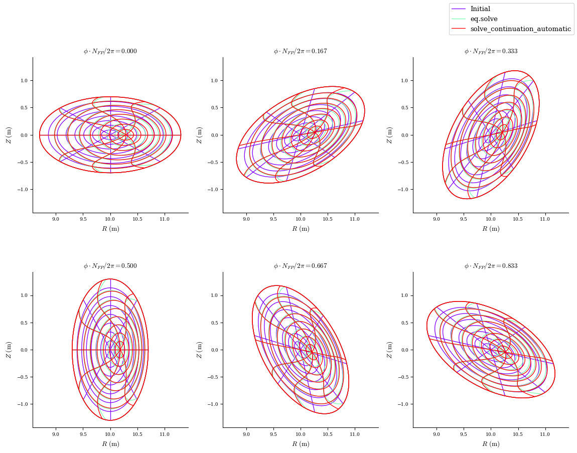
../../_images/notebooks_tutorials_basic_equilibrium_27_0.png

If we compute the normalized force balance error for each case, we see that using the continuation method gives ~20% lower error, indicating a better solution. For more complex equilibria this difference will often be much larger, which is why the continuation method is usually recommended.

[13]:

f1 = (
    eq1.compute("<|F|>_vol")["<|F|>_vol"]
    / eq1.compute("<|grad(|B|^2)|/2mu0>_vol")["<|grad(|B|^2)|/2mu0>_vol"]
)
f2 = (
    eqf[-1].compute("<|F|>_vol")["<|F|>_vol"]
    / eqf[-1].compute("<|grad(|B|^2)|/2mu0>_vol")["<|grad(|B|^2)|/2mu0>_vol"]
)
print(f"Force error after eq.solve(): {f1:.4e}")
print(f"Force error after solve_continuation_autmatic: {f2:.4e}")

Force error after eq.solve(): 9.2327e-03
Force error after solve_continuation_autmatic: 7.2373e-03