Zernike Polynomial Evaluation
This notebook compares different methods for evaluating the radial part of the Zernike polynomials, in terms of both speed and accuracy
The two primary methods we consider are direct polynomial evaluation using Horner’s method and an evaluation scheme based on a recurrence relation for Jacobi polynomials.
The radial part of the Zernike polynomials is given by
Because the coefficient of rho is made up of entirely integer operations, it can be evaluated quickly and exactly to arbitrary orders (recall that python natively supports arbitrary length integer arithmetic). These coefficients can then be evaluated using Horner’s method. This is done in the zernike_radial_poly function.
The other approach uses the fact that the above equation can be written as
Where \(P_{n}^{\alpha, \beta}\) is a Jacobi polynomial. This allows us to use stable recurrence relations for the Jacobi polynomials, as is done in the zernike_radial function.
[1]:
import sys
import os

sys.path.insert(0, os.path.abspath("."))
sys.path.append(os.path.abspath("../../"))
[ ]:
import numpy as np
import mpmath
import matplotlib
import matplotlib.pyplot as plt
from desc.basis import (
    polyder_vec,
    ZernikePolynomial,
    zernike_radial,
    zernike_radial_coeffs,
    zernike_radial_poly,
)
[3]:
basis = ZernikePolynomial(L=50, M=50, spectral_indexing="ansi", sym="cos")
r = np.linspace(0, 1, 1000)
Here we time the evaluation for a basis set containing 676 modes on a grid of 1000 points, for derivative orders 0 through 3. (note the block_until_ready is needed to get accurate timing with jax)
[4]:
print("zernike_radial, 0th derivative")
%time zr0 = zernike_radial(r[:,np.newaxis], basis.modes[:,0], basis.modes[:,1], 0).block_until_ready()
print("zernike_radial, 1st derivative")
%time zr1 = zernike_radial(r[:,np.newaxis], basis.modes[:,0], basis.modes[:,1], 1).block_until_ready()
print("zernike_radial, 2nd derivative")
%time zr2 = zernike_radial(r[:,np.newaxis], basis.modes[:,0], basis.modes[:,1], 2).block_until_ready()
print("zernike_radial, 3rd derivative")
%time zr3 = zernike_radial(r[:,np.newaxis], basis.modes[:,0], basis.modes[:,1], 3).block_until_ready()
zernike_radial, 0th derivative
CPU times: user 870 ms, sys: 47.3 ms, total: 917 ms
Wall time: 689 ms
zernike_radial, 1st derivative
CPU times: user 716 ms, sys: 27.3 ms, total: 743 ms
Wall time: 276 ms
zernike_radial, 2nd derivative
CPU times: user 1.1 s, sys: 5.68 ms, total: 1.11 s
Wall time: 399 ms
zernike_radial, 3rd derivative
CPU times: user 1.32 s, sys: 29.8 ms, total: 1.35 s
Wall time: 412 ms
[5]:
print("zernike_radial_poly, 0th derivative")
%time zp0 = zernike_radial_poly(r[:,np.newaxis], basis.modes[:,0], basis.modes[:,1], dr=0)
print("zernike_radial_poly, 1st derivative")
%time zp1 = zernike_radial_poly(r[:,np.newaxis], basis.modes[:,0], basis.modes[:,1], dr=1)
print("zernike_radial_poly, 2nd derivative")
%time zp2 = zernike_radial_poly(r[:,np.newaxis], basis.modes[:,0], basis.modes[:,1], dr=2)
print("zernike_radial_poly, 3rd derivative")
%time zp3 = zernike_radial_poly(r[:,np.newaxis], basis.modes[:,0], basis.modes[:,1], dr=3)
zernike_radial_poly, 0th derivative
CPU times: user 1min 53s, sys: 387 ms, total: 1min 53s
Wall time: 1min 52s
zernike_radial_poly, 1st derivative
CPU times: user 1min 57s, sys: 169 ms, total: 1min 58s
Wall time: 1min 57s
zernike_radial_poly, 2nd derivative
CPU times: user 1min 53s, sys: 188 ms, total: 1min 53s
Wall time: 1min 52s
zernike_radial_poly, 3rd derivative
CPU times: user 1min 52s, sys: 220 ms, total: 1min 52s
Wall time: 1min 51s
We see that the implementation using Jacobi polynomial recurrence relation is significantly faster, despite the overhead from the JAX just-in-time compiler
For accuracy comparison, we will also evaluate the Zernike radial polynomials in extended precision (100 digits of accuracy) and treat this as the “true” value.
[6]:
mpmath.mp.dps = 100
c = zernike_radial_coeffs(basis.modes[:, 0], basis.modes[:, 1], exact=True)

print("zernike_radial_exact, 0th derivative")
%time zt0 = np.array([np.asarray(mpmath.polyval(list(ci), r), dtype=float) for ci in c]).T
print("zernike_radial_exact, 1st derivative")
%time zt1 = np.array([np.asarray(mpmath.polyval(list(ci), r), dtype=float) for ci in polyder_vec(c,1)]).T
print("zernike_radial_exact, 2nd derivative")
%time zt2 = np.array([np.asarray(mpmath.polyval(list(ci), r), dtype=float) for ci in polyder_vec(c,2)]).T
print("zernike_radial_exact, 3rd derivative")
%time zt3 = np.array([np.asarray(mpmath.polyval(list(ci), r), dtype=float) for ci in polyder_vec(c,3)]).T
zernike_radial_exact, 0th derivative
CPU times: user 1min 45s, sys: 196 ms, total: 1min 45s
Wall time: 1min 44s
zernike_radial_exact, 1st derivative
CPU times: user 1min 41s, sys: 119 ms, total: 1min 41s
Wall time: 1min 41s
zernike_radial_exact, 2nd derivative
CPU times: user 1min 41s, sys: 258 ms, total: 1min 41s
Wall time: 1min 41s
zernike_radial_exact, 3rd derivative
CPU times: user 1min 42s, sys: 55.7 ms, total: 1min 42s
Wall time: 1min 41s
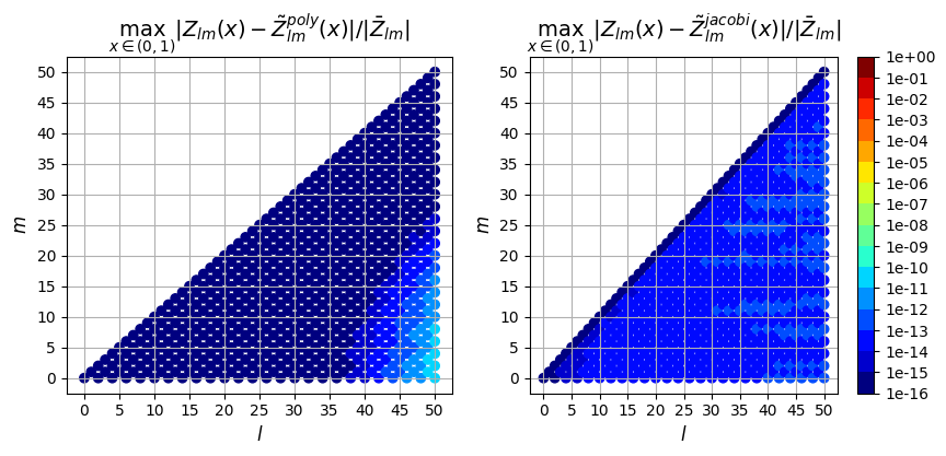
Next we can plot the error resulting from the two evaluation methods (polynomial evaluation and jacobi recurrence relation) vs the true solution computed in exact arithmetic. We plot the max absolute error as well as the max relative error over \(\rho \in (0,1)\) for each derivative order.
[7]:
cmap = plt.cm.jet  # define the colormap
# extract all colors from the .jet map
cmaplist = [cmap(i) for i in range(cmap.N)]

# create the new map
cmap = matplotlib.colors.LinearSegmentedColormap.from_list(
    "Custom cmap", cmaplist, cmap.N
)

# define the bins and normalize
bounds = np.logspace(-16, 0, 17)
norm = matplotlib.colors.BoundaryNorm(bounds, cmap.N)
Absolute Error
0th derivative
[8]:
fig, ax = plt.subplots(1, 2, squeeze=True, figsize=(10, 4))
im = ax[0].scatter(
    basis.modes[:, 0],
    basis.modes[:, 1],
    c=np.max(abs(zp0 - zt0), axis=0),
    norm=norm,
    cmap=cmap,
)
im = ax[1].scatter(
    basis.modes[:, 0],
    basis.modes[:, 1],
    c=np.max(abs(zr0 - zt0), axis=0),
    norm=norm,
    cmap=cmap,
)
cbar = fig.colorbar(im, ticks=bounds)
cbar.ax.set_yticklabels(["{:.0e}".format(foo) for foo in bounds])
ax[0].grid(True)
ax[1].grid(True)
ax[0].set_xticks(np.arange(0, 55, 5))
ax[0].set_yticks(np.arange(0, 55, 5))
ax[1].set_xticks(np.arange(0, 55, 5))
ax[1].set_yticks(np.arange(0, 55, 5))
ax[0].set_xlabel("$l$", fontsize=12)
ax[0].set_ylabel("$m$", fontsize=12)
ax[1].set_xlabel("$l$", fontsize=12)
ax[1].set_ylabel("$m$", fontsize=12)
ax[0].set_title(
    "$\max_{x \in (0,1)} |Z_{lm}(x) - \\tilde{Z}_{lm}^{poly}(x)|$", fontsize=14
)
ax[1].set_title(
    "$\max_{x \in (0,1)} |Z_{lm}(x) - \\tilde{Z}_{lm}^{jacobi}(x)|$", fontsize=14
);

1st derivative
[9]:
fig, ax = plt.subplots(1, 2, squeeze=True, figsize=(10, 4))
im = ax[0].scatter(
    basis.modes[:, 0],
    basis.modes[:, 1],
    c=np.max(abs(zp1 - zt1), axis=0),
    norm=norm,
    cmap=cmap,
)
im = ax[1].scatter(
    basis.modes[:, 0],
    basis.modes[:, 1],
    c=np.max(abs(zr1 - zt1), axis=0),
    norm=norm,
    cmap=cmap,
)
cbar = fig.colorbar(im, ticks=bounds)
cbar.ax.set_yticklabels(["{:.0e}".format(foo) for foo in bounds])
ax[0].grid(True)
ax[1].grid(True)
ax[0].set_xticks(np.arange(0, 55, 5))
ax[0].set_yticks(np.arange(0, 55, 5))
ax[1].set_xticks(np.arange(0, 55, 5))
ax[1].set_yticks(np.arange(0, 55, 5))
ax[0].set_xlabel("$l$", fontsize=12)
ax[0].set_ylabel("$m$", fontsize=12)
ax[1].set_xlabel("$l$", fontsize=12)
ax[1].set_ylabel("$m$", fontsize=12)
ax[0].set_title(
    "$\max_{x \in (0,1)} |\\frac{dZ_{lm}(x)}{dx} - \\frac{d\\tilde{Z}_{lm}^{poly}(x)}{dx}|$",
    fontsize=14,
)
ax[1].set_title(
    "$\max_{x \in (0,1)} |\\frac{dZ_{lm}(x)}{dx} - \\frac{d\\tilde{Z}_{lm}^{jacobi}(x)}{dx}|$",
    fontsize=14,
);

2nd derivative
[10]:
fig, ax = plt.subplots(1, 2, squeeze=True, figsize=(10, 4))
im = ax[0].scatter(
    basis.modes[:, 0],
    basis.modes[:, 1],
    c=np.max(abs(zp2 - zt2), axis=0),
    norm=norm,
    cmap=cmap,
)
im = ax[1].scatter(
    basis.modes[:, 0],
    basis.modes[:, 1],
    c=np.max(abs(zr2 - zt2), axis=0),
    norm=norm,
    cmap=cmap,
)
cbar = fig.colorbar(im, ticks=bounds)
cbar.ax.set_yticklabels(["{:.0e}".format(foo) for foo in bounds])
ax[0].grid(True)
ax[1].grid(True)
ax[0].set_xticks(np.arange(0, 55, 5))
ax[0].set_yticks(np.arange(0, 55, 5))
ax[1].set_xticks(np.arange(0, 55, 5))
ax[1].set_yticks(np.arange(0, 55, 5))
ax[0].set_xlabel("$l$", fontsize=12)
ax[0].set_ylabel("$m$", fontsize=12)
ax[1].set_xlabel("$l$", fontsize=12)
ax[1].set_ylabel("$m$", fontsize=12)
ax[0].set_title(
    "$\max_{x \in (0,1)} |\\frac{d^2 Z_{lm}(x)}{dx^2} - \\frac{d^2 \\tilde{Z}_{lm}^{poly}(x)}{dx^2}|$",
    fontsize=14,
)
ax[1].set_title(
    "$\max_{x \in (0,1)} |\\frac{d^2 Z_{lm}(x)}{dx^2} - \\frac{d^2 \\tilde{Z}_{lm}^{jacobi}(x)}{dx^2}|$",
    fontsize=14,
);

3rd derivative
[11]:
fig, ax = plt.subplots(1, 2, squeeze=True, figsize=(10, 4))
im = ax[0].scatter(
    basis.modes[:, 0],
    basis.modes[:, 1],
    c=np.max(abs(zp3 - zt3), axis=0),
    norm=norm,
    cmap=cmap,
)
im = ax[1].scatter(
    basis.modes[:, 0],
    basis.modes[:, 1],
    c=np.max(abs(zr3 - zt3), axis=0),
    norm=norm,
    cmap=cmap,
)
cbar = fig.colorbar(im, ticks=bounds)
cbar.ax.set_yticklabels(["{:.0e}".format(foo) for foo in bounds])
ax[0].grid(True)
ax[1].grid(True)
ax[0].set_xticks(np.arange(0, 55, 5))
ax[0].set_yticks(np.arange(0, 55, 5))
ax[1].set_xticks(np.arange(0, 55, 5))
ax[1].set_yticks(np.arange(0, 55, 5))
ax[0].set_xlabel("$l$", fontsize=12)
ax[0].set_ylabel("$m$", fontsize=12)
ax[1].set_xlabel("$l$", fontsize=12)
ax[1].set_ylabel("$m$", fontsize=12)
ax[0].set_title(
    "$\max_{x \in (0,1)} |\\frac{d^3 Z_{lm}(x)}{dx^3} - \\frac{d^3 \\tilde{Z}_{lm}^{poly}(x)}{dx^3}|$",
    fontsize=14,
)
ax[1].set_title(
    "$\max_{x \in (0,1)} |\\frac{d^3 Z_{lm}(x)}{dx^3} - \\frac{d^3 \\tilde{Z}_{lm}^{jacobi}(x)}{dx^3}|$",
    fontsize=14,
);

Relative Error
0th derivative
[12]:
fig, ax = plt.subplots(1, 2, squeeze=True, figsize=(10, 4))
im = ax[0].scatter(
    basis.modes[:, 0],
    basis.modes[:, 1],
    c=np.max(abs(zp0 - zt0), axis=0) / np.mean(abs(zt0)),
    norm=norm,
    cmap=cmap,
)
im = ax[1].scatter(
    basis.modes[:, 0],
    basis.modes[:, 1],
    c=np.max(abs(zr0 - zt0), axis=0) / np.mean(abs(zt0)),
    norm=norm,
    cmap=cmap,
)
cbar = fig.colorbar(im, ticks=bounds)
cbar.ax.set_yticklabels(["{:.0e}".format(foo) for foo in bounds])
ax[0].grid(True)
ax[1].grid(True)
ax[0].set_xticks(np.arange(0, 55, 5))
ax[0].set_yticks(np.arange(0, 55, 5))
ax[1].set_xticks(np.arange(0, 55, 5))
ax[1].set_yticks(np.arange(0, 55, 5))
ax[0].set_xlabel("$l$", fontsize=12)
ax[0].set_ylabel("$m$", fontsize=12)
ax[1].set_xlabel("$l$", fontsize=12)
ax[1].set_ylabel("$m$", fontsize=12)
ax[0].set_title(
    "$\max_{x \in (0,1)} |Z_{lm}(x) - \\tilde{Z}_{lm}^{poly}(x)| / |\\bar{Z}_{lm}|$",
    fontsize=14,
)
ax[1].set_title(
    "$\max_{x \in (0,1)} |Z_{lm}(x) - \\tilde{Z}_{lm}^{jacobi}(x)| / |\\bar{Z}_{lm}|$",
    fontsize=14,
);
1st derivative
[13]:
fig, ax = plt.subplots(1, 2, squeeze=True, figsize=(10, 4))
im = ax[0].scatter(
    basis.modes[:, 0],
    basis.modes[:, 1],
    c=np.max(abs(zp1 - zt1), axis=0) / np.mean(abs(zt1)),
    norm=norm,
    cmap=cmap,
)
im = ax[1].scatter(
    basis.modes[:, 0],
    basis.modes[:, 1],
    c=np.max(abs(zr1 - zt1), axis=0) / np.mean(abs(zt1)),
    norm=norm,
    cmap=cmap,
)
cbar = fig.colorbar(im, ticks=bounds)
cbar.ax.set_yticklabels(["{:.0e}".format(foo) for foo in bounds])
ax[0].grid(True)
ax[1].grid(True)
ax[0].set_xticks(np.arange(0, 55, 5))
ax[0].set_yticks(np.arange(0, 55, 5))
ax[1].set_xticks(np.arange(0, 55, 5))
ax[1].set_yticks(np.arange(0, 55, 5))
ax[0].set_xlabel("$l$", fontsize=12)
ax[0].set_ylabel("$m$", fontsize=12)
ax[1].set_xlabel("$l$", fontsize=12)
ax[1].set_ylabel("$m$", fontsize=12)
ax[0].set_title(
    "$\max_{x \in (0,1)} |\\frac{dZ_{lm}(x)}{dx} - \\frac{d\\tilde{Z}_{lm}^{poly}(x)}{dx}| / |\\bar{Z}'_{lm}|$",
    fontsize=14,
)
ax[1].set_title(
    "$\max_{x \in (0,1)} |\\frac{dZ_{lm}(x)}{dx} - \\frac{d\\tilde{Z}_{lm}^{jacobi}(x)}{dx}|/ |\\bar{Z}'_{lm}|$",
    fontsize=14,
);

2nd derivative
[14]:
fig, ax = plt.subplots(1, 2, squeeze=True, figsize=(10, 4))
im = ax[0].scatter(
    basis.modes[:, 0],
    basis.modes[:, 1],
    c=np.max(abs(zp2 - zt2), axis=0) / np.mean(abs(zt2)),
    norm=norm,
    cmap=cmap,
)
im = ax[1].scatter(
    basis.modes[:, 0],
    basis.modes[:, 1],
    c=np.max(abs(zr2 - zt2), axis=0) / np.mean(abs(zt2)),
    norm=norm,
    cmap=cmap,
)
cbar = fig.colorbar(im, ticks=bounds)
cbar.ax.set_yticklabels(["{:.0e}".format(foo) for foo in bounds])
ax[0].grid(True)
ax[1].grid(True)
ax[0].set_xticks(np.arange(0, 55, 5))
ax[0].set_yticks(np.arange(0, 55, 5))
ax[1].set_xticks(np.arange(0, 55, 5))
ax[1].set_yticks(np.arange(0, 55, 5))
ax[0].set_xlabel("$l$", fontsize=12)
ax[0].set_ylabel("$m$", fontsize=12)
ax[1].set_xlabel("$l$", fontsize=12)
ax[1].set_ylabel("$m$", fontsize=12)
ax[0].set_title(
    "$\max_{x \in (0,1)} |\\frac{d^2Z_{lm}(x)}{dx^2} - \\frac{d^2\\tilde{Z}_{lm}^{poly}(x)}{dx^2}| / |\\bar{Z}''_{lm}|$",
    fontsize=14,
)
ax[1].set_title(
    "$\max_{x \in (0,1)} |\\frac{d^2Z_{lm}(x)}{dx^2} - \\frac{d^2\\tilde{Z}_{lm}^{jacobi}(x)}{dx^2}|/ |\\bar{Z}''_{lm}|$",
    fontsize=14,
);

3rd derivative
[15]:
fig, ax = plt.subplots(1, 2, squeeze=True, figsize=(10, 4))
im = ax[0].scatter(
    basis.modes[:, 0],
    basis.modes[:, 1],
    c=np.max(abs(zp3 - zt3), axis=0) / np.mean(abs(zt3)),
    norm=norm,
    cmap=cmap,
)
im = ax[1].scatter(
    basis.modes[:, 0],
    basis.modes[:, 1],
    c=np.max(abs(zr3 - zt3), axis=0) / np.mean(abs(zt3)),
    norm=norm,
    cmap=cmap,
)
cbar = fig.colorbar(im, ticks=bounds)
cbar.ax.set_yticklabels(["{:.0e}".format(foo) for foo in bounds])
ax[0].grid(True)
ax[1].grid(True)
ax[0].set_xticks(np.arange(0, 55, 5))
ax[0].set_yticks(np.arange(0, 55, 5))
ax[1].set_xticks(np.arange(0, 55, 5))
ax[1].set_yticks(np.arange(0, 55, 5))
ax[0].set_xlabel("$l$", fontsize=12)
ax[0].set_ylabel("$m$", fontsize=12)
ax[1].set_xlabel("$l$", fontsize=12)
ax[1].set_ylabel("$m$", fontsize=12)
ax[0].set_title(
    "$\max_{x \in (0,1)} |\\frac{d^3Z_{lm}(x)}{dx^3} - \\frac{d^3\\tilde{Z}_{lm}^{poly}(x)}{dx^3}| / |\\bar{Z}'''_{lm}|$",
    fontsize=14,
)
ax[1].set_title(
    "$\max_{x \in (0,1)} |\\frac{d^3Z_{lm}(x)}{dx^3} - \\frac{d^3\\tilde{Z}_{lm}^{jacobi}(x)}{dx^3}|/ |\\bar{Z}'''_{lm}|$",
    fontsize=14,
);

So in addition to being faster, the evaluation using the Jacobi recurrence relation is also significantly more accurate as the mode numbers increase, keeping absolute error less than \(10^{-5}\) and relative error less than \(10^{-9}\), while directly evaluating the polynomial leads to errors greater than 100% for large \(l\)