desc.plotting.plot_section
- desc.plotting.plot_section(eq, name, grid=None, log=False, normalize=None, ax=None, return_data=False, compute_kwargs=None, **kwargs)Source
Plot Poincare sections.
- Parameters:
eq (Equilibrium) – Object from which to plot.
name (str) – Name of variable to plot.
grid (Grid, optional) – Grid of coordinates to plot at.
log (bool, optional) – Whether to use a log scale.
normalize (str, optional) – Name of the variable to normalize
nameby. Default is None.ax (matplotlib AxesSubplot, optional) – Axis to plot on.
return_data (bool) – If True, return the data plotted as well as fig,ax
compute_kwargs (dict, optional) – Additional keyword arguments to pass to
eq.compute.**kwargs (dict, optional) –
Specify properties of the figure, axis, and plot appearance e.g.:
plot_X(figsize=(4,6),label="your_label")
Valid keyword arguments are:
figsize: tuple of length 2, the size of the figure (to be passed to matplotlib)component: str, one of [None, ‘R’, ‘phi’, ‘Z’], For vector variables, which element to plot. Default is the norm of the vector.title_fontsize: integer, font size of the titlexlabel_fontsize: float, fontsize of the xlabelylabel_fontsize: float, fontsize of the ylabelcmap: str, matplotlib colormap scheme to use, passed to ax.contourflevels: int or array-like, passed to contourf. Ifname="|F|_normalized"andlog=True, default isnp.logspace(-6, 0, 7). Otherwise the default (None) uses the min/max values of the data.phi: float, int or array-like. Toroidal angles to plot. If an integer, plot that number equally spaced in [0,2pi/NFP). Default 1 for axisymmetry and 6 for non-axisymmetryfill: bool, Whether the contours are filled, i.e. whether to use contourf or contour. Default tofill=True
- Returns:
fig (matplotlib.figure.Figure) – Figure being plotted to.
ax (matplotlib.axes.Axes or ndarray of Axes) – Axes being plotted to.
plot_data (dict) – Dictionary of the data plotted, only returned if
return_data=True
Examples
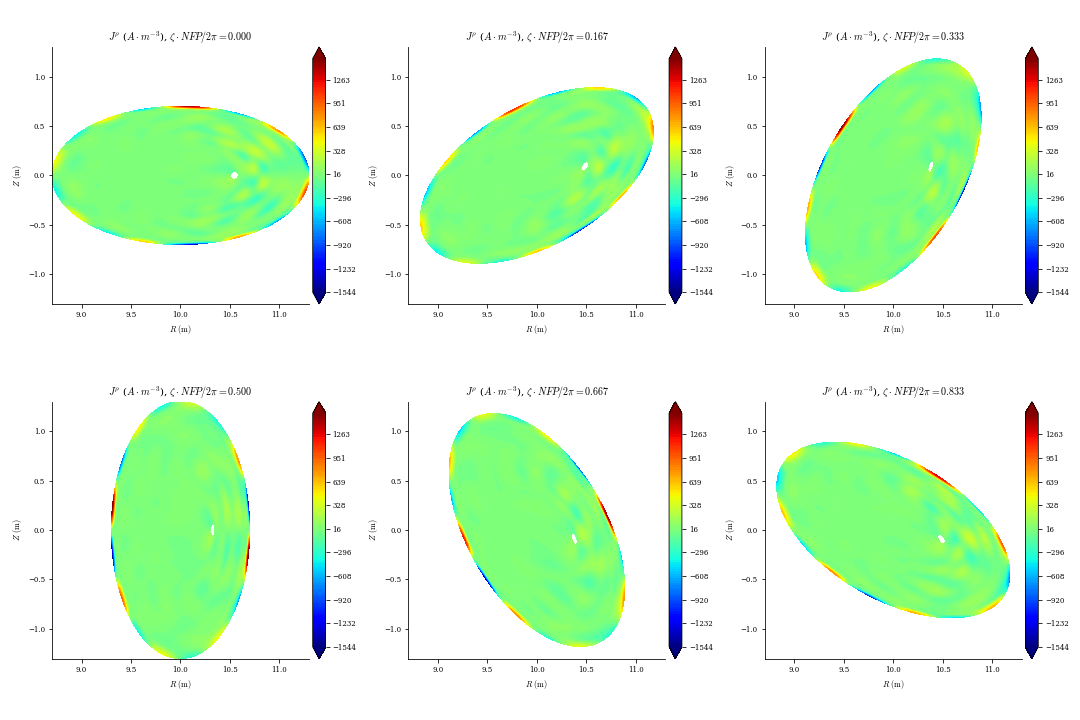
from desc.plotting import plot_section
fig, ax = plot_section(eq, "J^rho")