Using a DESC Equilibrium Output

import sys
import os

sys.path.insert(0, os.path.abspath("."))
sys.path.append(os.path.abspath("../../../"))

Loading in a DESC Equilibrium

DESC saves its output files as .h5 files, which can be loaded using the load function contained in the desc.io module

import desc.io

In DESC, equilibrium solutions are stored as Equilibrium objects, which contain the spectral coefficients of the solved equilibrium as well as the last-closed-flux-surface used to solve the equilibrium, the pressure and iota profiles, and other quantities that define the equilibrium.

Often in DESC, a continuation method is employed to solve for equilibria where a sequence of related equilibria are computed until the final resolution and input parameters are reached. When calling DESC from the command line, this sequence of Equilibrium objects are stored inside an EquilibriaFamily object, which essentially acts as a list of Equilibrium objects with some extra functionality to aid in the continuation method.

We will load in the solution to the HELIOTRON example input file we solved in the previous notebook now.

eq_fam = desc.io.load("HELIOTRON_output.h5")
print(type(eq_fam))

DESC version 0.7.2+334.g1fe6b36e.dirty,using JAX backend, jax version=0.4.1, jaxlib version=0.4.1, dtype=float64
Using device: CPU, with 9.80 GB available memory
<class 'desc.equilibrium.equilibrium.EquilibriaFamily'>

As you can see, the object we just loaded in is an EquilibriaFamily. We can check to see how many equilibria this family contains (3, each corresponding to a different step in the continuation method outlined in the HELIOTRON input file).

len(eq_fam)

8

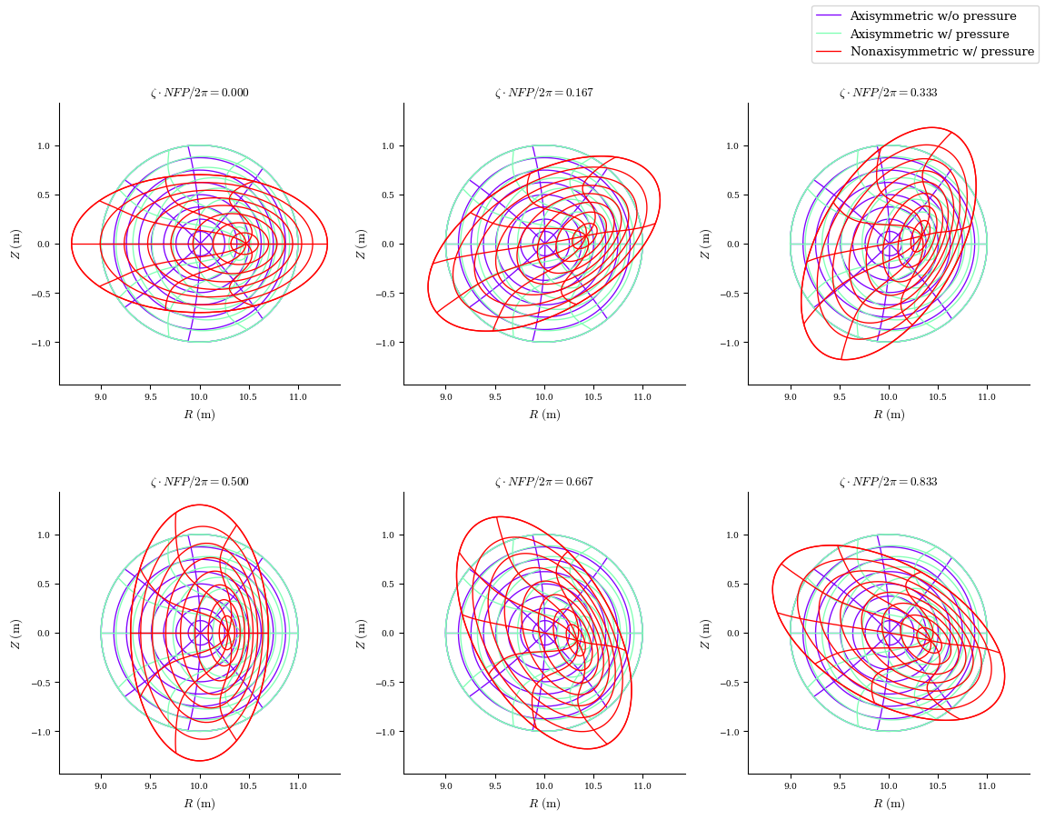
We can visualize the different equilibria with the plot_comparison function, which plots flux surfaces and the contours of constant straight field-line poloidal angle \(\vartheta=\theta+\lambda\) for multiple equilibria.

%matplotlib inline
from desc.plotting import plot_comparison

fig, ax = plot_comparison(
    eqs=[eq_fam[1], eq_fam[3], eq_fam[-1]],
    labels=[
        "Axisymmetric w/o pressure",
        "Axisymmetric w/ pressure",
        "Nonaxisymmetric w/ pressure",
    ],
)

Computing Quantities from a DESC Equilibrium

Now let’s focus on a single equilibrium. We can choose the final solution by indexing the last element of eq_fam

eq = eq_fam[-1]
print(type(eq))

<class 'desc.equilibrium.equilibrium.Equilibrium'>

Notice now we have an Equilibrium object, not an EquilibriaFamily. Printing an Equilibrium will list some information about it

print(eq)

Equilibrium at 0x7fb46d9e26a0 (L=12, M=12, N=3, NFP=19.0, sym=1, spectral_indexing=ansi)

Here we can see that this equilibrium solution has 19 field periods (NFP=19) and is represented with a Fourier-Zernike spectral basis with radial resolution of L=8, poloidal resolution of M=8, and toroidal resolution of N=3. It is stellarator symmetric (sym=1), and the spectral indexing scheme used for the Zernike Polynomial basis was the ansi indexing (for more information on the indexing schemes see the DESC documentation).

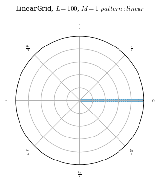
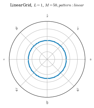
Grids in DESC are objects from the desc.grid module. We typically want to plot at linearly spaced points, so we will use the LinearGrid class to make a 1-dimensional grid of points linearly spaced in \(\rho\).

grid.nodes shows the points in the grid, each element being \((\rho,\theta,\zeta)\). Notice our grid is an array of points from \(\rho=0\) to \(\rho=1\) equally spaced, all at \(\theta=\zeta=0\).

from desc.grid import LinearGrid

grid_1d = LinearGrid(L=100)  # 101 linearly-spaced radial grid points
grid_1d.nodes[:10, :]  # show the first 10

array([[0.  , 0.  , 0.  ],
       [0.01, 0.  , 0.  ],
       [0.02, 0.  , 0.  ],
       [0.03, 0.  , 0.  ],
       [0.04, 0.  , 0.  ],
       [0.05, 0.  , 0.  ],
       [0.06, 0.  , 0.  ],
       [0.07, 0.  , 0.  ],
       [0.08, 0.  , 0.  ],
       [0.09, 0.  , 0.  ]])

We can visualize the grid using the plot_grid function.

from desc.plotting import plot_grid

plot_grid(grid_1d);

Equilibrium objects have a compute method which can be used to compute many useful quantities (a full list of which can be found in the DESC docs) that are commonly needed from an equilibrium.

The compute method takes as arguments the name (as a string) of the desired quantity and the grid you wish the quantity to be computed on. It then returns a dictionary containing that quantity, as well as all the intermediate quantities needed to compute the desired quantity.

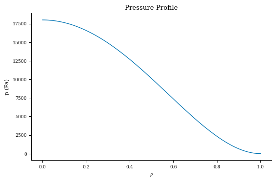
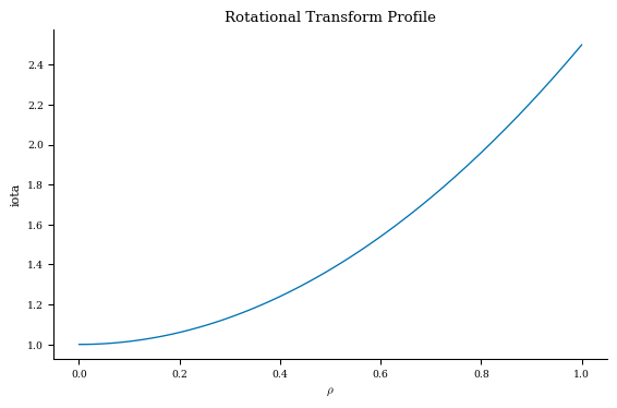
As an example, let’s plot the pressure and rotational transform profiles of this equilibrium.

pressure_data = eq.compute("p", grid=grid_1d)
iota_data = eq.compute("iota", grid=grid_1d)

pressure_data.keys()

dict_keys(['Te', 'ne', 'Ti', 'Zeff', 'p'])

iota_data.keys()

dict_keys(['rho', 'psi_r', 'iota'])

Notice that the returned dictionary for iota has more than just iota as a key. Generally, eq.compute will return the desired quantity along with each of its dependencies needed to calculate that quantity. Don’t rely on this, to ensure that you get all the quantities you need, it is better to pass in explicitly each quantity, for example you want both p and p_r, you must call eq.compute(["p","p_r"]).

Let’s plot the profiles now:

import matplotlib.pyplot as plt

p = pressure_data["p"]
iota = iota_data["iota"]

plt.figure()
plt.plot(grid_1d.nodes[:, 0], p)
plt.title("Pressure Profile")
plt.xlabel(r"$\rho$")
plt.ylabel("p (Pa)")

plt.figure()
plt.plot(grid_1d.nodes[:, 0], iota)
plt.title("Rotational Transform Profile")
plt.xlabel(r"$\rho$")
plt.ylabel("iota")

Text(0, 0.5, 'iota')

Now let’s compute the magnetic field strength on the \(\rho=0.5\) surface.

When making the grid we will specify that we want poloidal and toroidal grid points using \(M\) and \(N\), but only at the \(\rho=0.5\) surface. Adding the NFP argument to the grid will ensure we have toroidal points only for a single field period.

import numpy as np

# integer inputs specify the number of grid points in that dimension
# float or ndarray of floats specify the coordinate values
grid_2d_05 = LinearGrid(rho=np.array(0.5), M=50, N=50, NFP=eq.NFP, endpoint=True)
plot_grid(grid_2d_05);

Notice now that we have grid points at \(\rho=0.5\) and \(0\leq\theta<2\pi\) and \(0\leq\zeta<\frac{2\pi}{NFP}\)

mod_B_data = eq.compute("|B|", grid=grid_2d_05)

We can look at the returned dictionary now and see that all the intermediate quantities necessary to calculate |B| are also returned (the magnetic field covariant and contravariant components, metric tensor elements, etc.)

mod_B_data.keys()

dict_keys(['rho', 'psi_r', 'iota', '0', 'R_r', 'Z_r', 'e_rho', 'R_t', 'Z_t', 'e_theta', 'R', 'R_z', 'Z_z', 'e_zeta', 'sqrt(g)', 'B0', 'lambda_z', 'B^theta', 'lambda_t', 'B^zeta', 'B', '|B|^2', '|B|'])

mod_B = mod_B_data["|B|"]

To plot this 2d data, it is important to understand that in DESC all quantities and grid points are by default in a single stack. If we look at the shape of grid_2d_05.nodes, we can see that it is 10,000 nodes (1 \(\rho\) coordinate x 100 \(\theta\) coordinates x 100 \(\zeta\) coordinates), each of length 3 \((\rho,\theta,\zeta)\). Similarly, mod_B is given at these 10,000 nodes.

grid_2d_05.nodes.shape

(10201, 3)

mod_B.shape

(10201,)

To plot this, we must reshape it into a 2D array as follows

# reshape to form grids for plotting
zeta = (
    grid_2d_05.nodes[:, 2]
    .reshape((grid_2d_05.num_theta, grid_2d_05.num_rho, grid_2d_05.num_zeta), order="F")
    .squeeze()
)
theta = (
    grid_2d_05.nodes[:, 1]
    .reshape((grid_2d_05.num_theta, grid_2d_05.num_rho, grid_2d_05.num_zeta), order="F")
    .squeeze()
)
mod_B = mod_B.reshape(
    (grid_2d_05.num_theta, grid_2d_05.num_rho, grid_2d_05.num_zeta), order="F"
)

# plot contours of |B| on the rho=0.5 surface
plt.contourf(zeta, theta, mod_B[:, 0, :], cmap="jet")
plt.xlabel(r"$\zeta$")
plt.ylabel(r"$\theta$")
plt.title(r"$|\mathbf{B}|$ on $\rho=0.5$ surface")

Text(0.5, 1.0, '$|\\mathbf{B}|$ on $\\rho=0.5$ surface')

Hopefully the process of computing quantities from a DESC equilibrium is clearer now. A full list of the quantities available for computation already in DESC is given in the DESC documentation

Plotting Utilities In DESC

For normal plotting needs, DESC has an extensive array of plotting utilities that can be used to quickly plot quantities of interest.

from desc.plotting import plot_1d, plot_2d, plot_3d, plot_section, plot_boozer_surface

fig, ax = plot_1d(eq, "p")  # default grid is linearly spaced in rho
fig, ax = plot_1d(eq, "iota")
fig, ax = plot_2d(eq, "|B|", grid=grid_2d_05)  # plot |B| on rho=0.5 surface

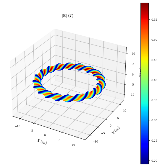
fig, ax = plot_3d(eq, "|B|")
# note that this example has 19 toroidal field periods

fig, ax = plot_section(eq, "|F|")  # plot force error

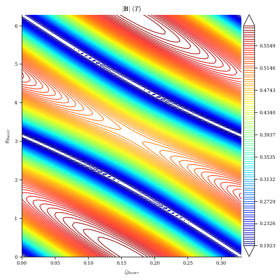
# |B| in Boozer coordinates on the rho=0.7 surface
fig, ax = plot_boozer_surface(
    eq, grid_plot=LinearGrid(rho=np.array(0.7), M=50, N=50, NFP=eq.NFP, endpoint=True)
)

Each of the plotting routines takes additional arguments that can be used to customize the appearance of the plots, full details can be found in the documentation.

Also note that each plotting function returns a handle to the Matplotlib figure and a numpy array of the axes used. These can then be further modified to customize the appearance of the plots.