Continuation method step by step
In this example we step through the continuation method step by step - starting from an axisymmetric vacuum configuration, adding 3D shaping, and then adding pressure.
If you have access to a GPU, uncomment the following two lines before any DESC or JAX related imports. You should see about an order of magnitude speed improvement with only these two lines of code!
[2]:
# from desc import set_device
# set_device("gpu")
As mentioned in DESC Documentation on performance tips, one can use compilation cache directory to reduce the compilation overhead time. Note: One needs to create jax-caches folder manually.
[ ]:
# import jax

# jax.config.update("jax_compilation_cache_dir", "../jax-caches")
# jax.config.update("jax_persistent_cache_min_entry_size_bytes", -1)
# jax.config.update("jax_persistent_cache_min_compile_time_secs", 0)
[3]:
%matplotlib inline
import numpy as np

from desc.equilibrium import Equilibrium
from desc.geometry import FourierRZToroidalSurface
from desc.objectives import (
    ObjectiveFunction,
    ForceBalance,
    get_fixed_boundary_constraints,
)
from desc.optimize import Optimizer
from desc.plotting import plot_1d, plot_section, plot_surfaces
from desc.profiles import PowerSeriesProfile
An NVIDIA GPU may be present on this machine, but a CUDA-enabled jaxlib is not installed. Falling back to cpu.
DESC version 0.13.0+702.ge6b8a02dc.dirty,using JAX backend, jax version=0.4.33, jaxlib version=0.4.33, dtype=float64
Using device: CPU, with 44.34 GB available memory
2D Equilibrium
We start by creating the surface object that represents the axisymmetric boundary.
[4]:
surface_2D = FourierRZToroidalSurface(
    R_lmn=np.array([10, -1]),  # boundary coefficients
    Z_lmn=np.array([1]),
    modes_R=np.array([[0, 0], [1, 0]]),  # [M, N] boundary Fourier modes
    modes_Z=np.array([[-1, 0]]),
    NFP=5,  # number of (toroidal) field periods (does not matter for 2D, but will for 3D solution)
)
Now we can initialize an Equilibrium with this boundary surface. By default, Equilibrium objects have pressure and net toroidal current profiles of 0 assigned. We also increase the resolution and use a collocation grid that oversamples by a factor of two.
[5]:
# axisymmetric & stellarator symmetric equilibrium
eq = Equilibrium(surface=surface_2D, sym=True)
eq.change_resolution(L=6, M=6, L_grid=12, M_grid=12)
Next we create our objective function, ForceBalance which will seek to make \(\mathbf{F} \equiv \mathbf{J} \times \mathbf{B} - \nabla p = 0\)
[6]:
objective = ObjectiveFunction(ForceBalance(eq=eq))
Next we need to specify the optimization constraints, which indicate what parameters that will remain fixed during the optimization process. For this fixed-boundary problem we can call the utility function get_fixed_boundary_constraints that returns a list of the desired constraints.
[7]:
constraints = get_fixed_boundary_constraints(eq=eq)
for c in constraints:
    print(c)
<desc.objectives.linear_objectives.FixBoundaryR object at 0x153a68890680>
<desc.objectives.linear_objectives.FixBoundaryZ object at 0x153a685f74d0>
<desc.objectives.linear_objectives.FixPsi object at 0x153a68546030>
<desc.objectives.linear_objectives.FixPressure object at 0x153a5f76bd10>
<desc.objectives.linear_objectives.FixCurrent object at 0x153a68547b30>
<desc.objectives.linear_objectives.FixSheetCurrent object at 0x153a5f5c6900>
Finally, we can solve the equilibrium with the objective and constraints specified above. We also chose an optimization algorithm by initializing an Optimizer object. The verbose=3 option will display output at each optimization step.
[8]:
# this is a port of scipy's trust region least squares algorithm but using JAX functions for better performance
optimizer = Optimizer("lsq-exact")
eq, solver_outputs = eq.solve(
    objective=objective, constraints=constraints, optimizer=optimizer, verbose=3
)
Building objective: force
Precomputing transforms
Timer: Precomputing transforms = 1.58 sec
Timer: Objective build = 1.97 sec
Building objective: lcfs R
Building objective: lcfs Z
Building objective: fixed Psi
Building objective: fixed pressure
Building objective: fixed current
Building objective: fixed sheet current
Building objective: self_consistency R
Building objective: self_consistency Z
Building objective: lambda gauge
Building objective: axis R self consistency
Building objective: axis Z self consistency
Timer: Objective build = 729 ms
Timer: Linear constraint projection build = 3.50 sec
Number of parameters: 27
Number of objectives: 98
Timer: Initializing the optimization = 6.24 sec

Starting optimization
Using method: lsq-exact
   Iteration     Total nfev        Cost      Cost reduction    Step norm     Optimality
       0              1          9.294e-03                                    1.350e-01
       1              2          1.709e-03      7.585e-03      2.108e-01      3.122e-02
       2              3          1.750e-04      1.534e-03      8.901e-02      1.071e-02
       3              4          3.711e-06      1.713e-04      5.145e-02      1.255e-03
       4              5          2.621e-07      3.449e-06      3.861e-02      3.428e-04
       5              6          1.749e-08      2.446e-07      1.658e-02      1.173e-04
       6              7          1.490e-10      1.734e-08      3.866e-03      8.023e-06
       7              8          8.859e-11      6.042e-11      8.400e-03      1.001e-05
       8              9          3.323e-13      8.826e-11      9.622e-04      4.061e-07
       9             11          6.377e-14      2.686e-13      9.001e-04      1.438e-07
      10             14          1.716e-15      6.205e-14      1.368e-04      1.775e-08
      11             16          1.540e-16      1.562e-15      6.484e-05      1.021e-08
      12             18          1.121e-17      1.427e-16      3.527e-05      2.280e-09
`gtol` condition satisfied.
         Current function value: 1.121e-17
         Total delta_x: 1.839e-01
         Iterations: 12
         Function evaluations: 18
         Jacobian evaluations: 13
Timer: Solution time = 3.89 sec
Timer: Avg time per step = 299 ms
==============================================================================================================
                                                                 Start  -->   End
Total (sum of squares):                                      9.294e-03  -->   1.121e-17,
Maximum absolute Force error:                                7.882e+04  -->   1.327e-02 (N)
Minimum absolute Force error:                                1.042e-11  -->   5.887e-07 (N)
Average absolute Force error:                                2.555e+04  -->   6.991e-04 (N)
Maximum absolute Force error:                                6.339e-03  -->   1.067e-09 (normalized)
Minimum absolute Force error:                                8.380e-19  -->   4.735e-14 (normalized)
Average absolute Force error:                                2.055e-03  -->   5.622e-11 (normalized)
R boundary error:                                            0.000e+00  -->   0.000e+00 (m)
Z boundary error:                                            0.000e+00  -->   0.000e+00 (m)
Fixed Psi error:                                             0.000e+00  -->   0.000e+00 (Wb)
Fixed pressure profile error:                                0.000e+00  -->   0.000e+00 (Pa)
Fixed current profile error:                                 0.000e+00  -->   0.000e+00 (A)
Fixed sheet current error:                                   0.000e+00  -->   0.000e+00 (~)
==============================================================================================================
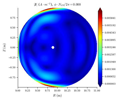
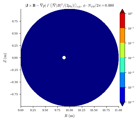
We can analyze the equilibrium solution using the available plotting routines. . Here we plot the magnitude of the total current density \(|\mathbf{J}|\) and the normalized force balance error. We expect both quantities to be low for this vacuum solution.
[9]:
plot_section(eq, "|J|")
plot_section(eq, "|F|", norm_F=True, log=True);
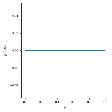
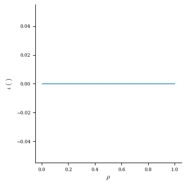
Since this is an axisymmetric vacuum equilibrium, there should be no pressure or rotational transform. We can plot both quantities as follows:
[10]:
plot_1d(eq, "p")
plot_1d(eq, "iota");
3D Equilibrium
Now we want to solve a stellarator vacuum equilibrium by perturbing the existing tokamak solution we already found. We start by creating a new surface to represent the 3D (non-axisymmetric) stellarator boundary.
[11]:
surface_3D = FourierRZToroidalSurface(
    R_lmn=np.array([10, -1, -0.3, 0.3]),  # boundary coefficients
    Z_lmn=np.array([1, -0.3, -0.3]),
    modes_R=np.array(
        [[0, 0], [1, 0], [1, 1], [-1, -1]]
    ),  # [M, N] boundary Fourier modes
    modes_Z=np.array([[-1, 0], [-1, 1], [1, -1]]),
    NFP=5,  # number of (toroidal) field periods
)
In the previous solution we did not use any toroidal Fourier modes because they were unnecessary for axisymmetry. Now we need to increase the toroidal resolution, and we will also increase the radial and poloidal resolutions as well. Again we oversample the collocation grid by a factor of two.
We will also update the resolution of the 3D surface to match the new resolution of the Equilibrium.
[12]:
eq.change_resolution(L=10, M=10, N=6, L_grid=20, M_grid=20, N_grid=12)
surface_3D.change_resolution(eq.L, eq.M, eq.N)
We need to initialize new instances of the objective and constraints. This is necessary because the original instances got built for a specific resolution during the previous 2D equilibrium solve, and are no longer compatible with the Equilibrium after increasing the resolution.
[13]:
objective = ObjectiveFunction(ForceBalance(eq=eq))
constraints = get_fixed_boundary_constraints(eq=eq)
Next is the boundary perturbation. In this step, we approximate the heliotron equilibrium solution from a 2nd-order Taylor expansion about the axisymmetric solution. This is possible thanks to the wealth of derivative information provided by automatic differentiation.
[14]:
eq.perturb(
    deltas={
        "Rb_lmn": surface_3D.R_lmn - eq.Rb_lmn,  # change in the R boundary coefficients
        "Zb_lmn": surface_3D.Z_lmn - eq.Zb_lmn,  # change in the Z boundary coefficients
    },
    objective=objective,  # perturb the solution such that J=0 is maintained
    constraints=constraints,  # same constraints used in the equilibrium solve
    order=2,  # use a 2nd-order Taylor expansion
    verbose=2,  # display timing data
);
Building objective: force
Precomputing transforms
Timer: Precomputing transforms = 1.03 sec
Timer: Objective build = 1.25 sec
Building objective: lcfs R
Building objective: lcfs Z
Building objective: fixed Psi
Building objective: fixed pressure
Building objective: fixed current
Building objective: fixed sheet current
Building objective: self_consistency R
Building objective: self_consistency Z
Building objective: lambda gauge
Building objective: axis R self consistency
Building objective: axis Z self consistency
Timer: Objective build = 722 ms
Perturbing Rb_lmn, Zb_lmn
Factorizing linear constraints
Timer: linear constraint factorize = 4.02 sec
Computing df
Timer: df computation = 7.72 sec
Factoring df
Timer: df/dx factorization = 37.4 ms
Computing d^2f
Timer: d^2f computation = 4.75 sec
Timer: Objective build = 1.60 ms
||dx||/||x|| =  3.838e-02
Timer: Total perturbation = 20.1 sec
[14]:
Equilibrium at 0x153a68ba8050 (L=10, M=10, N=6, NFP=5, sym=True, spectral_indexing=ansi)
We now have an approximation of the stellarator equilibrium from the tokamak solution! Let us look at the 3D surfaces and rotational transform profile to check that the perturbation actually updated the solution:
[15]:
plot_surfaces(eq)
plot_1d(eq, "iota");
The surfaces match the heliotron boundary we want and there is non-zero rotational transform as expected. But the equilibrium error is now large because the perturbed solution is only an approximation to the true equilibrium:
[16]:
plot_section(eq, "|F|", norm_F=True, log=True);
We can re-solve the equilibrium using the new 3D boundary constraint. This should converge in only a few Newton iterations because we are starting from a good initial guess.
[17]:
eq, solver_outputs = eq.solve(
    objective=objective,  # solve JxB-grad(p)=0
    constraints=constraints,  # fixed-boundary constraints
    optimizer=optimizer,  # we can use the same optimizer as before
    ftol=1e-2,  # stopping tolerance on the function value
    xtol=1e-4,  # stopping tolerance on the step size
    gtol=1e-6,  # stopping tolerance on the gradient
    maxiter=20,  # maximum number of iterations
    verbose=3,  # display output at each iteration
)
Building objective: self_consistency R
Building objective: self_consistency Z
Building objective: lambda gauge
Building objective: axis R self consistency
Building objective: axis Z self consistency
Timer: Objective build = 26.8 ms
Timer: Linear constraint projection build = 348 ms
Number of parameters: 1011
Number of objectives: 6050
Timer: Initializing the optimization = 395 ms

Starting optimization
Using method: lsq-exact
   Iteration     Total nfev        Cost      Cost reduction    Step norm     Optimality
       0              1          7.712e-02                                    1.351e-01
       1              2          1.330e-03      7.579e-02      8.667e-02      1.773e-02
       2              3          8.914e-05      1.241e-03      6.466e-02      3.997e-03
       3              4          2.510e-05      6.403e-05      9.845e-02      2.085e-03
       4              5          1.204e-05      1.306e-05      1.045e-01      1.463e-03
       5              6          2.321e-06      9.723e-06      9.350e-02      7.256e-04
       6              7          4.612e-08      2.274e-06      1.932e-02      7.465e-05
       7              8          4.675e-09      4.144e-08      6.092e-03      3.095e-05
       8              9          2.313e-09      2.361e-09      3.511e-03      2.178e-05
       9             10          7.758e-10      1.537e-09      2.763e-03      1.367e-05
      10             11          1.046e-10      6.712e-10      1.689e-03      5.095e-06
Optimization terminated successfully.
`xtol` condition satisfied.
         Current function value: 1.046e-10
         Total delta_x: 3.084e-01
         Iterations: 10
         Function evaluations: 11
         Jacobian evaluations: 11
Timer: Solution time = 20.5 sec
Timer: Avg time per step = 1.87 sec
==============================================================================================================
                                                                 Start  -->   End
Total (sum of squares):                                      7.712e-02  -->   1.046e-10,
Maximum absolute Force error:                                2.937e+06  -->   1.531e+02 (N)
Minimum absolute Force error:                                5.101e+00  -->   1.829e-05 (N)
Average absolute Force error:                                5.107e+04  -->   1.229e+00 (N)
Maximum absolute Force error:                                2.362e-01  -->   1.232e-05 (normalized)
Minimum absolute Force error:                                4.103e-07  -->   1.471e-12 (normalized)
Average absolute Force error:                                4.108e-03  -->   9.888e-08 (normalized)
R boundary error:                                            0.000e+00  -->   0.000e+00 (m)
Z boundary error:                                            0.000e+00  -->   0.000e+00 (m)
Fixed Psi error:                                             0.000e+00  -->   0.000e+00 (Wb)
Fixed pressure profile error:                                0.000e+00  -->   0.000e+00 (Pa)
Fixed current profile error:                                 0.000e+00  -->   0.000e+00 (A)
Fixed sheet current error:                                   0.000e+00  -->   0.000e+00 (~)
==============================================================================================================
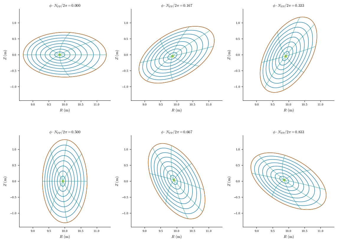
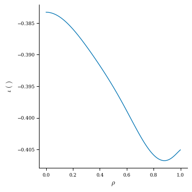
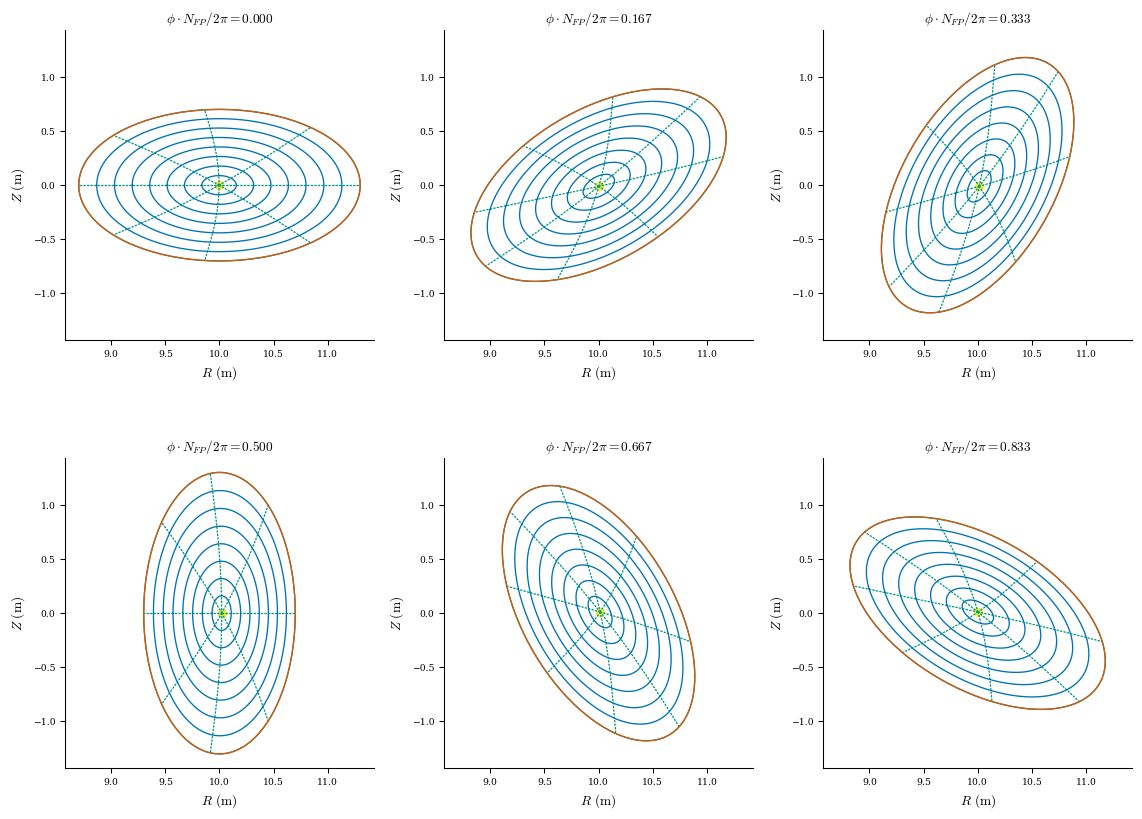
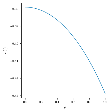
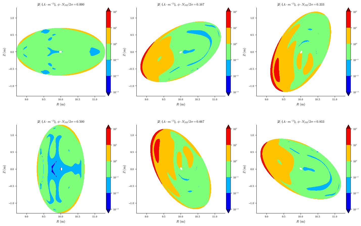
We can analyze our final solution using the same plotting commands as before. Note that the flux surfaces and rotational transform profile only had small corrections compared to the perturbed solution, but the equilibrium error was significantly improved.
[18]:
plot_surfaces(eq)
plot_1d(eq, "iota")
plot_section(eq, "|J|", log=True)
plot_section(eq, "|F|", norm_F=True, log=True);
Finite beta stellarator
We’ve solved for a vacuum stellarator, but what if we now want to look at what happens at finite beta? We can simply apply a pressure perturbation.
[19]:
from desc.objectives import ForceBalance

objective = ObjectiveFunction(ForceBalance(eq=eq))
constraints = get_fixed_boundary_constraints(eq=eq, profiles=True)
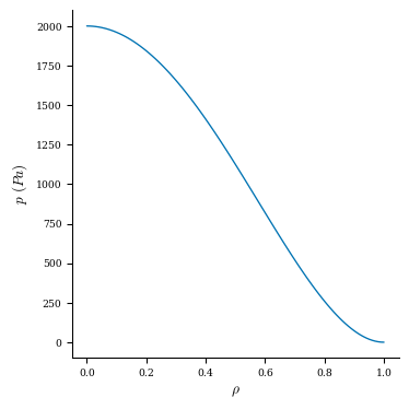
Next we’ll make our desired pressure profile, corresponding to a profile of the form \(p(\rho) = 2000(1 - 2 \rho^2 + \rho^4) ~\text{Pa}\)
[20]:
from desc.profiles import PowerSeriesProfile

pressure = PowerSeriesProfile([2000, 0, -4000, 0, 2000])
pressure.change_resolution(eq.L)
Now, we will perturb our equilibrium’s pressure coefficients \(p_l\) to match those of the target pressure
[21]:
eq.perturb(
    deltas={"p_l": pressure.params - eq.p_l},  # change in the pressure coefficients
    objective=objective,  # perturb the solution such that JxB-grad(p)=0 is maintained
    constraints=constraints,  # same constraints used in the equilibrium solve
    order=2,  # use a 2nd-order Taylor expansion
    verbose=2,  # display timing data
);
Building objective: force
Precomputing transforms
Timer: Precomputing transforms = 65.2 ms
Timer: Objective build = 88.6 ms
Building objective: lcfs R
Building objective: lcfs Z
Building objective: fixed Psi
Building objective: fixed pressure
Building objective: fixed current
Building objective: fixed sheet current
Building objective: self_consistency R
Building objective: self_consistency Z
Building objective: lambda gauge
Building objective: axis R self consistency
Building objective: axis Z self consistency
Timer: Objective build = 130 ms
Perturbing p_l
Factorizing linear constraints
Timer: linear constraint factorize = 357 ms
Computing df
Timer: df computation = 35.2 ms
Factoring df
Timer: df/dx factorization = 549 us
Computing d^2f
Timer: d^2f computation = 9.14 ms
Timer: Objective build = 1.62 ms
||dx||/||x|| =  6.322e-02
Timer: Total perturbation = 4.78 sec
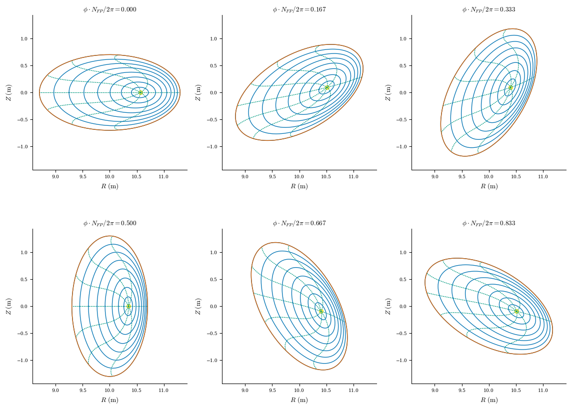
We can see that the axis has moved due to the Shafranov shift, and the pressure profile is now nonzero. The force balance error is significantly larger, however.
[22]:
plot_surfaces(eq)
plot_1d(eq, "p")
plot_section(eq, "|F|", norm_F=True, log=True);
[23]:
eq, solver_outputs = eq.solve(
    objective=objective,  # solve JxB-grad(p)=0
    constraints=constraints,  # fixed-boundary and profile constraints
    optimizer=optimizer,  # we can use the same optimizer as before
    ftol=1e-2,  # stopping tolerance on the function value
    xtol=1e-4,  # stopping tolerance on the step size
    gtol=1e-6,  # stopping tolerance on the gradient
    maxiter=75,  # maximum number of iterations
    verbose=3,  # display output at each iteration
)
Building objective: self_consistency R
Building objective: self_consistency Z
Building objective: lambda gauge
Building objective: axis R self consistency
Building objective: axis Z self consistency
Timer: Objective build = 31.1 ms
Timer: Linear constraint projection build = 375 ms
Number of parameters: 1011
Number of objectives: 6050
Timer: Initializing the optimization = 424 ms

Starting optimization
Using method: lsq-exact
   Iteration     Total nfev        Cost      Cost reduction    Step norm     Optimality
       0              1          6.506e-02                                    1.958e-01
       1              2          5.514e-04      6.451e-02      1.079e-01      9.209e-03
       2              3          3.161e-04      2.353e-04      1.144e-01      6.339e-03
       3              5          1.788e-04      1.373e-04      6.797e-02      8.907e-03
       4              6          2.383e-05      1.549e-04      6.313e-02      1.848e-03
       5              8          5.615e-06      1.822e-05      2.795e-02      1.445e-03
       6             10          5.806e-07      5.034e-06      1.861e-02      3.927e-04
       7             12          1.344e-07      4.463e-07      8.325e-03      8.911e-05
       8             14          1.129e-07      2.143e-08      4.212e-03      1.984e-05
       9             16          1.112e-07      1.746e-09      2.146e-03      5.100e-06
Optimization terminated successfully.
`xtol` condition satisfied.
         Current function value: 1.112e-07
         Total delta_x: 2.001e-01
         Iterations: 9
         Function evaluations: 16
         Jacobian evaluations: 10
Timer: Solution time = 40.3 sec
Timer: Avg time per step = 4.03 sec
==============================================================================================================
                                                                 Start  -->   End
Total (sum of squares):                                      6.506e-02  -->   1.112e-07,
Maximum absolute Force error:                                1.028e+06  -->   5.783e+02 (N)
Minimum absolute Force error:                                3.598e+01  -->   1.156e-02 (N)
Average absolute Force error:                                5.637e+04  -->   7.404e+01 (N)
Maximum absolute Force error:                                8.266e-02  -->   4.651e-05 (normalized)
Minimum absolute Force error:                                2.894e-06  -->   9.295e-10 (normalized)
Average absolute Force error:                                4.533e-03  -->   5.955e-06 (normalized)
R boundary error:                                            0.000e+00  -->   0.000e+00 (m)
Z boundary error:                                            0.000e+00  -->   0.000e+00 (m)
Fixed Psi error:                                             0.000e+00  -->   0.000e+00 (Wb)
Fixed pressure profile error:                                0.000e+00  -->   0.000e+00 (Pa)
Fixed current profile error:                                 0.000e+00  -->   0.000e+00 (A)
Fixed sheet current error:                                   0.000e+00  -->   0.000e+00 (~)
==============================================================================================================
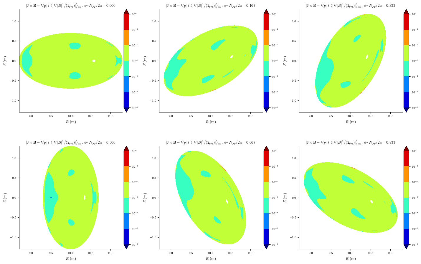
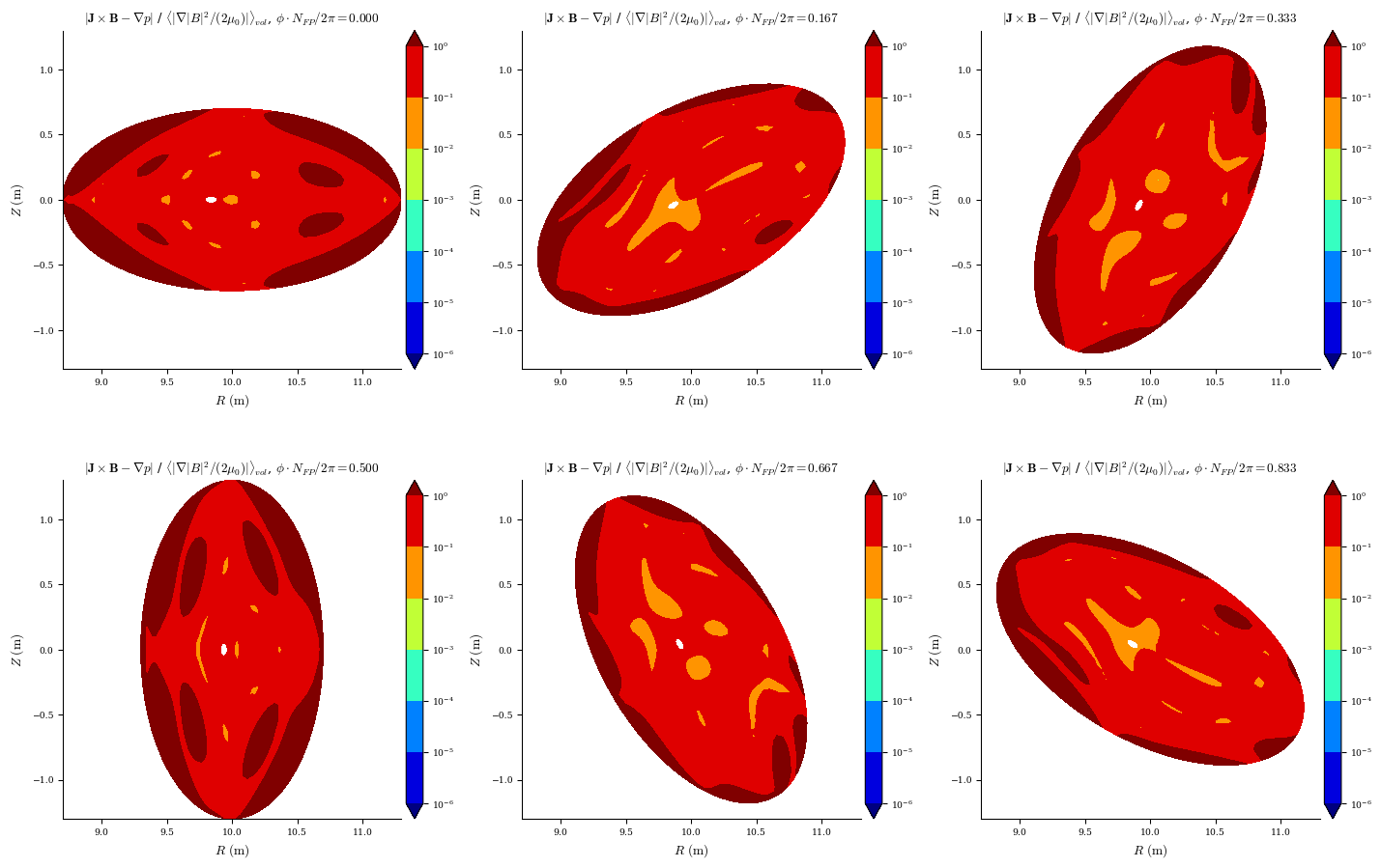
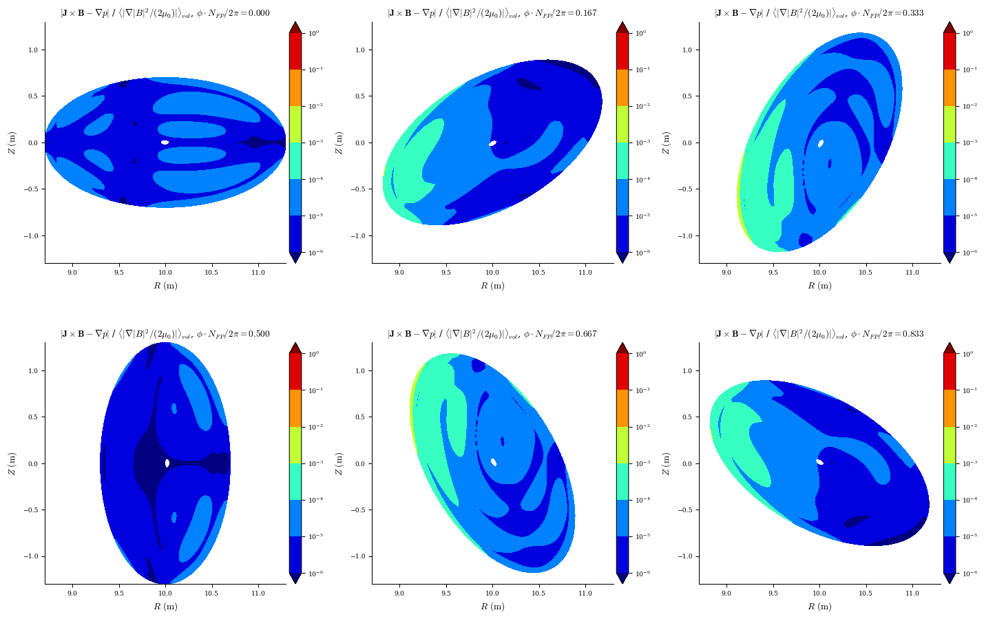
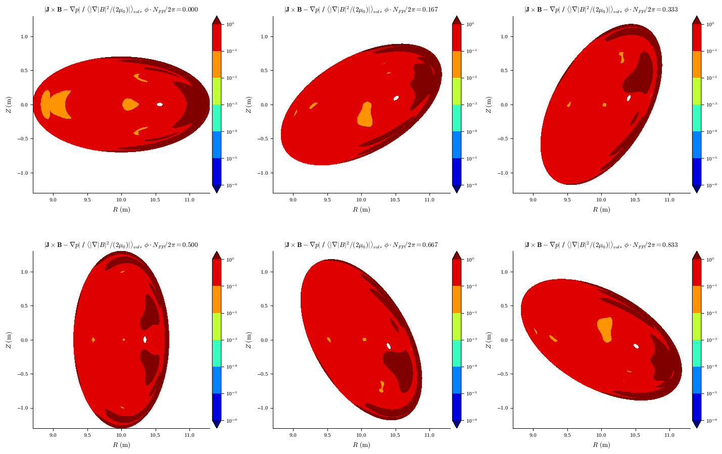
After re-solving, we find the force blance residuals are much lower, less than 1% normalized errors throughout the volume:
[24]:
plot_section(eq, "|F|", norm_F=True, log=True);